"The journey of a thousand miles begins with a single step."
- An Ancient Chinese proverb.
Fractal and Chaos mathematics relies heavily on numerical data and images created using computers. In this chapter we will give a behind the scenes look at some of the algorithms used in generating some of these programs such as FractaSketch™ and MandelMovie™, as well as demonstrate ways you can create your own programs using languages: C, Basic, PostScript™ and Mathematica™.
| 7.1
Drawing self-similar fractals: Internal algorithms and data structures
of FractaSketch™ |
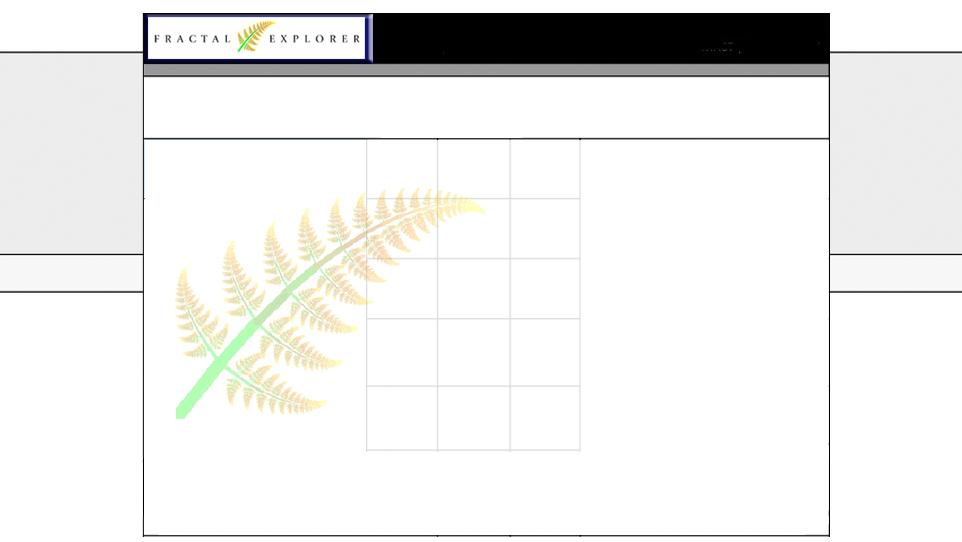
Figure 7.1 A flower hedge made from the recursion of FractaSketch™.
7.1.1 Introduction
A lot of effort was done to make FractaSketch fast and useful. This section describes some of the internal algorithms and ideas behind the implementation of FractaSketch on the Macintosh. These are illustrated with simple mathematical formulas and code fragments in C and 68000 assembly code. I assume a smattering of knowledge of these languages, of the Macintosh Toolbox, and of high school mathematics. The program was developed in Think C (formerly Lightspeed C).
This chapter is divided into six parts: In the first part I explain the basic algorithm and its data structures. In the second part I relate this to Lindenmayer systems, a method for describing plant structures that has a lot in common with the way FractaSketch works. In the third part I explain various techniques for drawing faster and more accurately. In the fourth part I describe a novel programming technique that solves a small problem in the implementation. This technique is not generally presented in programming books, but it is powerful and easy to use so I include it here. In the fifth part, I explain how to calculate the dimension of a self-similar fractal, both exactly (by formula) and approximately (by counting pixels). In the sixth part I give a detailed description of the file formats that FractaSketch writes and can read.
7.1.2 The basic algorithm
The fractals drawn by FractaSketch are all self-similar. That is, a small part of the fractal, if magnified, looks exactly like the original fractal.
To draw a self-similar fractal, the main drawing routine is recursive, that is, it calls itself. This is a very natural way to draw self-similar fractals: since the program calls itself, the smaller parts of the fractal will of course be identical in form to the original fractal.
7.2.1 Turtlegraphics
The drawing routine works in a two-dimensional plane. It draws using a well-known technique called "turtlegraphics". It is as if there were a "turtle" on the plane, carrying a drawing pen, that listens to the following commands:
Forward(n) Go forward n pixels.
Back(n) Go backward n pixels.
Left(d) Turn left d degrees.
Right(d) Turn right d degrees.
Penup() Lift the pen up (stop drawing).
Pendown() Put the pen down (start drawing).
These commands do exactly what you expect them to do. They are very powerful: any self-similar fractal made of line segments can be drawn easily as a sequence of turtlegraphics commands. The program keeps track of the turtle's position, velocity, and direction with the following structure:
typedef
struct {
fixed x, y;
/* Position */
fixed vx, vy; /* Velocity */
angle direc;
/* Direction */
}
TURTLE_STATE;
This structure is the turtle state. The types fixed and angle are defined later on.
With turtlegraphics commands, a simple recursive routine to draw the Koch snowflake looks like this in C:
draw_snowflake(level,
length)
int
level; /* Level of complexity of the fractal */
float
length; /* Length of the fractal */
{
if (level<=0) {
Forward(length);
} else {
draw_snowflake(level-1, length/3);
Left(60.0);
draw_snowflake(level-1, length/3);
Right(120.0);
draw_snowflake(level-1, length/3);
Left(60.0);
draw_snowflake(level-1, length/3);
}
}
This uses the turtlegraphics commands Forward, Left, and Right. The draw_snowflake routine calls itself four times. It does not go into an infinite loop because the level variable is decremented: each recursive call draws a simpler fractal, until the level reaches zero, which draws a single line segment.
It would be tedious to have to write a new program each time you want to draw a different fractal. This is where FractaSketch helps you. It allows you to define a simple template (the "seed" of a fractal; see the FractaSketch user manual) graphically and to draw it in many ways, without writing a single line of code. In fact, the program is usable even if the keyboard is broken. [1] The template is automatically interpreted as a sequence of turtlegraphics commands. How this is done is explained in the next section.
2.2 The fractal state
All the information about a fractal is kept in a data structure called the "fractal state". The main drawing routine, DrawFractal, reads the information in the fractal state to draw a particular fractal. When a fractal is saved in a file, what is actually saved is the fractal state. If you have more than one fractal on the screen (each in its own window), the program keeps track of all of them by giving each its own fractal state. It switches state to draw another template. The fractal state data structure is defined like this:
#define
MAXPTS 100 /* Maximum number of points
in template */
#define
DIMSTR 10 /* Length of dimension string
*/
#define MAXNAME 40
/* Length of file name */
typedef
struct {
/* Information
per template */
int numpt;
/* Number of points in template
*/
angle
ddraworg; /* Origin direction
*/
double
xdraworg, ydraworg; /* Origin point */
double
drawscale; /* Drawing scale */
int drawmode;
/* Drawing
pen mode */
double
drawsize; /* Drawing pen size */
int propflag;
/* Proportional/constant flag */
int lastlevel;
/* Level
of last drawing */
char dimstr[DIMSTR];
/* Dimension
of fractal */
char filename[MAXNAME];
/* Current file name for open and save */
/* Information
per segment of a template: */
fixpoint fplst[MAXPTS]; /*
Coordinates of point, latched on grid */
Point plst[MAXPTS]; /* Coordinates of point, free */
angle absalst[MAXPTS]; /* Absolute Angle list */
angle relalst[MAXPTS]; /* Relative Angle list:
r[i]=a[i]-a[i-1] */
fixed slst[MAXPTS]; /* Segment length */
int filst[MAXPTS]; /* Index to other template */
int backflags[MAXPTS]; /* Forward/backward drawing
flag */
int botflags[MAXPTS]; /* Yes/no recursive drawing
flag */
int invflags[MAXPTS]; /* Normal/invert drawing flag
*/
int leftflags[MAXPTS]; /* Left/right drawing flag */
int propflags[MAXPTS]; /* Proportional/constant
thickness flag */
/* Other information: */
/* ... Window information ... */
/* ... Fractal editing information ... */
The global constant MAXPTS defines the maximum number of points in a template, and hence also the maximum number of segments (= points - 1). The fixpoint type is a point whose coordinates are fixed point numbers. The angle type gives the angle in units of 1/48th of a degree. Both of these types are explained in more detail later on.
The template is made up of line segments. Each of these segments can be given ten possible meanings: four orientations, four orientations with inverted drawing (invert everything under the pen instead of drawing black), solid black ("solid" means no recursive drawing), and solid white (an invisible line segment, used to make disjoint templates). These orientations correspond to particular values of the flags arrays in the fractal state. When creating the template, the orientations are shown on the screen by drawing the segments with an arrowhead and a shading.
3 The relationship with Lindenmayer
systems
It is possible to increase the variety of fractals that can be drawn beyond that of FractaSketch by adding new parameters to the ones that already exist. For readers wishing to explore this, I highly recommend the book The Algorithmic Beauty of Plants by Lindenmayer and Prusinkiewicz (Springer-Verlag). This book is clearly written and profusely illustrated, it does not shirk from defining intricate grammar formalisms, the Lindenmayer systems or L-systems.
L-systems are a mathematical way of describing plant development. An L-system describes a plant as a string, or sequence of characters, in a given language. Each character has a particular meaning, for example, a stem with a particular length, a branching point from which the plant grows in more than one direction, a change of the growth direction of the plant, a change of the character of plant growth, e.g., from stems to buds and flowers, and so forth.
Not all character strings correspond to plants. An L-system is used to generate valid strings from a set of rewriting rules and an initial string. For example, the following L-system represents the Koch snowflake:
Initial string: F
Rewrite rule: F -> F+F-F+F
The character "F" corresponds to "Move forward",
"+" to "Turn left
by
![]() degrees", and "-"
to "Turn right by
degrees", and "-"
to "Turn right by
![]() degrees". Successive generations are:
degrees". Successive generations are:
F
F+F-F+F
F+F-F+F+F+F-F+F-F+F-F+F+F+F-F+F
F+F-F+F+F+F-F+F-F+F-F+F+F+F-F+F+F+F-F+F+F+F-F+F-F+F-F+F+F+F-F+F-F+F-F+F+F+F-F+F-F+F-F+F+F+F-F+F+F+F-F+F+F+F-F+F-F+F-F+F+F+F-F+F
...
If these strings are interpreted as graphic commands, they will draw the Koch snowflake. A grammar rule in an L-system corresponds to a template in FractaSketch. This example barely scratches the surface of the possibilities that have been explored with L-systems.
The power of FractaSketch is that the manipulation of grammar rules is done graphically and interactively. The question of how to describe graphically the more powerful formalism of L-systems is still unanswered. An answer to this question would significantly increase the power of FractaSketch while keeping it easy to understand and simple to use.
4 Techniques to increase speed
and accuracy
This section describes some of the techniques used to increase the performance of FractaSketch. First, I explain the representation of points and why it is efficient. Then, I explain the techniques used to make turtlegraphics go faster. Finally, I describe the memory management scheme and the trade-off between memory usage and speed of window refreshing.
4.1 How points are represented
Points in the plane are represented
as two fixed point numbers of 32-bits each. Each fixed point number has
a 16-bit integer part and a 16-bit fractional part. This means that each
pixel on the screen is divided up into
![]() parts, so the resolution is
parts, so the resolution is
![]() , or about
, or about
![]() of a pixel. Because of high drawing
accuracy, high zoom, and fast arithmetic, this is a good trade-off for a
Macintosh based on a 68000 processor. As machines become faster and faster,
64-bit floating point numbers might become a reasonable alternative.
of a pixel. Because of high drawing
accuracy, high zoom, and fast arithmetic, this is a good trade-off for a
Macintosh based on a 68000 processor. As machines become faster and faster,
64-bit floating point numbers might become a reasonable alternative.
Points are always represented internally with this accuracy. They are rounded to the nearest integer only when they are drawn. This guarantees a high quality drawing. All "fringe effects" are due to the round-off inherent in pixel-based display (beginning and ending points must be on a pixel), not to the internal representation of pixels. It is possible to use the "clipping" facility of the Toolbox to reduce this error. The idea is to draw a very long line and to clip the line to a small box that corresponds exactly to the part that has to be displayed. The only problem with this technique is that it is very slow.
The 16-bit integer part means
that points range from
![]() to
to
![]() , or
, or
![]() to
to
![]() .
[2]
The size of a drawing is limited by the
screen size, which is typically something like 512 times 342 (for a Macintosh
Classic internal screen) and can range up to 1280 times 1024 or even bigger.
This means that the maximum zoom-in factor will be around 32 to 64.
.
[2]
The size of a drawing is limited by the
screen size, which is typically something like 512 times 342 (for a Macintosh
Classic internal screen) and can range up to 1280 times 1024 or even bigger.
This means that the maximum zoom-in factor will be around 32 to 64.
4.2 Fast turtlegraphics
To do turtlegraphics well,
one has to do the Forward
![]() and the Left
and the Left
![]() operations as fast as possible. The Forward
operations as fast as possible. The Forward
![]() operation involves the following calculation:
operation involves the following calculation:
xnew
= xold + (vx * n);
ynew
= yold + (vy * n);
where (vx,vy) is the direction vector, that is, we have:
vx
= cos(direc);
vy
= sin(direc);
where direc is the direction angle. The Left(d) operation involves the following calculation:
direc
= direc + d;
vx
= cos(direc);
vy
= sin(direc);
In other words, to do Forward well, we need to be able to add and multiply fast, and to do Left well, we need to be able to add and calculate sines and cosines fast. Adding two fixed point numbers quickly is easy: standard integer addition will add them in a single instruction. The following two sections discuss multiplication and trigonometry, which are harder to do quickly.
4.2.1 How to go forward quickly
To draw a self-similar fractal with turtlegraphics, one needs to do a lot of multiplications. The Macintosh Toolbox provides a fixed point multiplication routine built in, called FixMul. From measurements, I found that the Toolbox calling overhead is quite high, which noticeably slows down the raw multiplication time. Therefore I wrote a version of FixMul, called FastFixMul, in 68000 assembly language. The Think C compiler accepts inline assembly language instructions with the asm statement, and it allows symbolic labels and C variables in the assembly code. Here is the routine:
#define
answer D0
#define
sign D1
#define
holdf1 A0
fixed
FastFixMul(f1, f2)
register
fixed f1, f2;
{
asm {
clr sign
/* Get f1 and f2; Set sign flag */
tst.l f1
bpl.s @posf1
neg.l f1
not sign
posf1: tst.l f2
bpl.s @posf2
neg.l f2
not sign
posf2: move.l f1,
answer /* Multiply low parts
(lf1*lf2) */
mulu f2,
answer
addi.l #32768,
answer
clr.w answer
swap answer
move.l f1,
holdf1 /* Multiply intermediate
(hf1*lf2) */
swap f1
tst.w f1
beq.s @hf1z1
mulu f2,f1
add.l f1,
answer
hf1z1: swap f2
/* Multiply intermediate
(lf1*hf2) */
tst.w f2
beq.s @hf2z
move.l holdf1,
f1
mulu f2,
f1
add.l f1,
answer
move.l holdf1,
f1 /* Multiply high parts
(hf1*hf2) */
swap f1
tst.w f1
beq.s @hf1z2
mulu f1,
f2
swap f2
clr.w f2
add.l f2,
answer
hf2z:
hf1z2: tst sign
/* Adjust sign of answer
*/
bpl.s @posans
neg.l answer
posans:
}
}
Fixed point numbers are 32-bit, and therefore fit nicely into the 68000's registers. This routine has two fixed point arguments, f1 and f2. It assumes that the function result (called answer) is stored in register D0 and that registers D1 and A0 are available as temporaries.
With this routine as the heart of the Forward operation, the main overhead is the line drawing time, that is, the time taken by the Toolbox routine LineTo. I did not replace this routine because it would be too complicated: LineTo automatically does clipping, takes the drawing mode and pensize into account, and properly interfaces with Quickdraw. The only way to make it faster would have been to write a routine to draw directly into screen memory, and this would have made the program non-portable.
4.2.2 How to turn quickly
To do the Left operation quickly, one has to be able to calculate sines and cosines quickly. I solved this problem by storing sines and cosines in a table, and doing simple table lookup when I needed their values. The table is declared as follows:
typedef
long angle; /* Angles are long integers */
#define
circ14 ((angle) 4320) /* 1/4-circle (90 degrees) */
fixed
sintab[circ14+1]; /* Table of sines */
It is enough to store the sines for a quarter-circle, since the other sines and the cosines can be derived easily from simple trigonometry:
sin(180
- x) = sin(x); /* Angles from 90
to 180 degrees */
sin(180
+ x) = - sin(x); /* Angles from 180 to 360 degrees */
sin(360
+ x) = sin(x); /* Angles more than
360 degrees */
cos(x)
= sin(90 - x); /* Angles from
0 to 90 degrees */
cos(180
- x) = - cos(x); /* Angles from 90 to 180 degrees */
cos(180
+ x) = - cos(x); /* Angles from 180 to 360 degrees */
cos(360
+ x) = cos(x); /* Angles more than
360 degrees */
Angles are represented as integers
of type angle, whose size is chosen
so that 4320 is
![]() degrees. This means that the unit
is
degrees. This means that the unit
is
![]() degree. Why did I chose this strange
value? First, the unit had to be as small as possible, so that the roundoff
error would be small. Second, the common angles of
degree. Why did I chose this strange
value? First, the unit had to be as small as possible, so that the roundoff
error would be small. Second, the common angles of
![]() degrees (square) and
degrees (square) and
![]() degrees (triangle) had to be exactly
representable. Third, the table of sines had to be as big as possible, given
the memory limitations of Think C. It turns out that the compiler only allowed
32 kilobytes of global data, which limits the table size to 8192 entries
(this is (32768 bytes) / (4 bytes per fixed point value)). Because the program
needs space for other global data, the biggest size that fits with the second
constraint is 4320.
degrees (triangle) had to be exactly
representable. Third, the table of sines had to be as big as possible, given
the memory limitations of Think C. It turns out that the compiler only allowed
32 kilobytes of global data, which limits the table size to 8192 entries
(this is (32768 bytes) / (4 bytes per fixed point value)). Because the program
needs space for other global data, the biggest size that fits with the second
constraint is 4320.
During program startup, the
table sintab has to be initialized.
On a Macintosh Plus this takes several seconds because the Toolbox sine
routine is rather slow (it works only in Extended precision, an 80-bit floating
point type). To shorten this time, I replaced the calls to the Toolbox sine
routine by the following sine routine which calculates sines from
![]() to
to
![]() degrees much more quickly:
degrees much more quickly:
#define
circ11 ((angle) 17280) /* Full circle (360 degrees) */
static
double c1=411774.832/circ11;
static
double c2=2708752.4/circ11/circ11/circ11;
static
double c3=5230709.3/circ11/circ11/circ11/circ11/circ11;
/*
Fast sine for angles from 0 to circ18 (45 degrees) */
/*
Returns 65536.0*sin(a) with maximum error 0.1 */
double
FastSine(a)
angle
a;
{
double x =
(double)a;
double xx = x*x;
return (x*(c1-xx*(c2-xx*c3)));
}
The values of the constants
c1, c2,
and c3 come from a reference book
on functional approximation. Sines from
![]() to
to
![]() degrees are obtained with the formula:
degrees are obtained with the formula:
sin(90
- x) = cos(x);
=
sqrt(1 - sin^2(x));
Square roots are very fast on the Mac: they execute in about the same time as a multiplication.
4.2.3 How to avoid cumulative
roundoff error during drawing
A complicated fractal consists
of a large number of short line segments. These line segments are all drawn
with the Forward or Back commands, which each updates the turtle's position.
Since the position is represented only approximately, there will be a small
error, the roundoff error, in the new position. This error has two causes: first, the position is only accurate
to about
![]() pixel, and second, the angle is
only accurate to
pixel, and second, the angle is
only accurate to
![]() degree. When the error reaches one
pixel it will become visible on the screen. If the fractal is complex, containing
thousands of line segments, it is likely that the error will become visible.
If the screen is zoomed in, the error becomes larger. If the fractal template contains s segments
and is drawn to level
degree. When the error reaches one
pixel it will become visible on the screen. If the fractal is complex, containing
thousands of line segments, it is likely that the error will become visible.
If the screen is zoomed in, the error becomes larger. If the fractal template contains s segments
and is drawn to level
![]() , then the total number of segments is
, then the total number of segments is
![]() . The cumulative roundoff error is therefore proportional to
. The cumulative roundoff error is therefore proportional to
![]() ). For example, a Koch snowflake curve has four segments. Drawing it at
level five results in
). For example, a Koch snowflake curve has four segments. Drawing it at
level five results in
![]() line segments.
line segments.
There is a simple technique
that reduces this roundoff from s
to s times n. For all practical purposes, this removes the error completely.
For the Koch snowflake example, the error is reduced from
![]() to
to
![]() times
times
![]() =
=
![]() , a reduction factor of about
, a reduction factor of about
![]() . For more complicated fractals, the reduction is even higher.
. For more complicated fractals, the reduction is even higher.
The technique is implemented in the drawing routine as follows: save the turtle state before drawing, then draw the fractal, then restore the state and move to the final position in a single Forward operation. This replaces the cumulative roundoff error of the whole drawing (which may have thousands of Forward operations) by the error of a single Forward operation. To implement this, two operations are added to the turtlegraphics package:
Savestate(&s) Copy the turtle state to s.
Restorestate(s)
Copy s to the turtle state.
In these two operations, s is a structure of type TURTLE_STATE and the ampersand "&" is a C operator that returns a reference (a pointer) to its argument. With these two operations, the technique is easy to program. The draw_snowflake routine given earlier becomes:
draw_snowflake(level,
length)
int
level; /* Level of complexity of the fractal */
float
length; /* Length of the fractal */
{
if (level<=0) {
Forward(length);
} else {
TURTLE_STATE
s;
Savestate(&s);
draw_snowflake(level-1, length/3);
Left(60.0);
draw_snowflake(level-1, length/3);
Right(120.0);
draw_snowflake(level-1, length/3);
Left(60.0);
draw_snowflake(level-1, length/3);
Restorestate(s);
Penup();
Forward(length);
Pendown();
}
}
The additional operations needed are shown in bold face type. The local variable s contains the turtle state. This variable is only allocated when level>0.
4.3 Memory management
When a window containing a fractal is partially covered and then uncovered, the uncovered part has to be redrawn. This process is called "refreshing the window". FractaSketch has two methods to refresh windows: either redraw the fractal in the window, or copy a saved image to the window. The first method uses almost no memory, but is very slow for complicated fractals. The second method uses lots of memory (for large windows this can be several hundred kilobytes or more), but is almost instantaneous. As long as enough memory is available, FractaSketch uses the second method. The decision which method to use is determined each time a fractal is drawn during execution. This means that closing unused windows during execution will allow the remaining windows to be refreshed quicker.
If you intend to do development of complex fractals on a big screen, performance will be greater if you increase the memory allocated to FractaSketch upon startup. This can be done by selecting the FractaSketch program from the Finder, doing GetInfo, and editing the memory partition size.
The maximum number of fractal windows that can be open at any one time is determined at launch time by the amount of available memory. A partition of 300 kilobytes allows about 10 windows to be open. One extra window can be opened for every 20 kilobytes added to the partition size. The smallest partition that works is about 150 kilobytes, which will allow a single fractal window to be opened.
5 The technique of "faking it"
If you hold down the mouse button and move the mouse, you will drag an outline of the fractal across the window. This seems simple enough, but to get it to work right requires a technique that is considered "state of the art" in programming language implementation. It is called abstract interpretation or symbolic execution and is usually associated with heavy mathematical machinery. Do not let this scare you--the idea is simple and easy to use. In fact, you have probably already used it without being aware of it.
The idea is this: You have a complicated program (like a fractal drawing program with lots and lots of ways to customize it). You would like to find out something about what you get when executing it, but without actually executing it. No sweat! Write a simple program that mimics the part of the big program that you are interested in. Then just execute the simple program. [3] There is only one rule to follow: the simple program must exactly mimic the big program.
How is this used in dragging an outline across the screen? When you drag the mouse, the program will draw over and over again a simple version of the fractal, so that you see what you are dragging. There is a problem, though: the program would like to draw as much as possible of the real fractal, but not too much or else redraw time would be too slow, and dragging would become a drag. The program has to draw the fractal at the highest drawing level that gives less than some maximum number of line segments (say, 50). This guarantees that as much as possible of the fractal will be redrawn while keeping redrawing fast.
To find out what level to draw the outline, there is a simple routine that "goes through the motions" of the full drawing routine DrawFractal, but only counts visible line segments. This routine is a simplified version of DrawFractal: all the parts that are needed to draw segments are removed, and only the parts needed to find out if a segment is visible or invisible are kept. Here it is:
/*
Count the number of visible segments with a given drawing level. */
/*
This routine does symbolic execution of the routine DrawFractal. */
int
CountSegments(level, visflag)
int
level;
register
int visflag;
{
register int vis;
register int i;
if (level==0) return visflag;
vis=0;
level-;
if (level>0)
for(i=1;i<numpt;i++)
vis += botflags[i]
? invflags[i]
: CountSegments(level, visflag^ invflags[i]);
else
for(i=1;i<numpt;i++)
vis += botflags[i]
? invflags[i]
: visflag^ invflags[i];
return vis;
}
Notice how this routine uses the arrays botflags and invflags defined in the fractal state. This routine is a lot simpler than DrawFractal, and a lot faster too, since it does not do any calculations or drawing. But it gets the job done: it counts the number of visible line segments for a given drawing level.
6 Calculating the fractal dimension
The single most interesting number that characterizes a fractal is its dimension. There are many definitions of dimensionality (see Mandelbrot's book The Fractal Geometry of Nature for a survey of the more important ones). A definition that works for a Euclidean space is the number of coordinates needed to specify the position of a point. For example, a plane is specified by two coordinates, an x and a y coordinate, so it has dimension two.
It is possible to generalize dimension to non-integer values. One's intuition about dimension then changes: dimension is no longer an indication of the number of coordinates, but a measure of a kind of extension or complexity of the shape. A square has more extension than a line segment, hence it has higher dimension (two instead of one). A Koch snowflake has more extension than a line segment, but less than a square. Hence, its dimension lies somewhere between one and two (it is about 1.2618).
One of the most powerful definitions of dimension is known as the Hausdorff-Besicovitch dimension. This definition is powerful because it assigns a dimension number to almost any set, whereas weaker definitions sometimes throw up their hands, so to speak, and give no answer.
A much weaker, but still very useful definition is called the similarity dimension. This definition only works for self-similar sets, and is easy to calculate when one knows how the sets are constructed. It is possible to prove that under some very general conditions, the similarity dimension, when it exists, is equal to the Hausdorff-Besicovitch dimension.
Two methods of calculating the dimension are implemented in FractaSketch. The first method (the "theoretical" method) calculates the similarity dimension from the fractal state. It uses the equation for similarity dimension given by Mandelbrot, and finds a numerical solution to this equation. The second method (the "empirical" method) gives an approximate value of the Hausdorff-Besicovitch dimension directly by drawing the fractal and counting how many "balls" are necessary to cover it. The number of "balls", as a function of the size of the ball, gives the dimension.
6.1 The theoretical method:
Calculating the similarity dimension
We would like to calculate
the similarity dimension of a fractal of which we know the template. The
template is a list of line segments and related information used to recursively
draw a fractal. The line segments have length
![]() , where
, where
![]() ranges from
ranges from
![]() to
to
![]() , where
, where
![]() is the number of segments in the template. The
is the number of segments in the template. The
![]() are normalized to the length of
the template: they are divided by the length
are normalized to the length of
the template: they are divided by the length
![]() of the template (the distance between
the first and the last point):
of the template (the distance between
the first and the last point):
![]()
For the Koch snowflake, each
![]() has value
has value
![]() and
and
![]() ranges from
ranges from
![]() to
to
![]() . The similarity dimension
. The similarity dimension
![]() satisfies the formula:
satisfies the formula:
![]()
For example, for the Koch snowflake this becomes:
![]()
Solving this equation gives:
![]()
In the general case, the
![]() have different values, so solving
the equation is not quite this easy as seen in Chapter 4. FractaSketch uses
a numerical method called Newton's
method seen in Chapter 6 or the Newton-Raphson method to find a solution.
This method is used to find a solution (a "root") of the equation:
have different values, so solving
the equation is not quite this easy as seen in Chapter 4. FractaSketch uses
a numerical method called Newton's
method seen in Chapter 6 or the Newton-Raphson method to find a solution.
This method is used to find a solution (a "root") of the equation:
![]()
where:
![]()
Newton's method works by iteration.
The process starts by guessing a value
![]() for the root. This value is improved
by running it through the formula:
for the root. This value is improved
by running it through the formula:
![]()
where
![]() is the derivative
of
is the derivative
of
![]() with respect to
with respect to
![]() , that is, it gives the slope of
, that is, it gives the slope of
![]() at position
at position
![]() . Simple calculus gives:
. Simple calculus gives:
![]()
where
![]() is the natural logarithm of
is the natural logarithm of
![]() .
.
The iteration continues until
![]() (the "error") is less
than some given number. FractaSketch gives dimensions to four decimals of
accuracy. It stops the iteration when the error is less than
(the "error") is less
than some given number. FractaSketch gives dimensions to four decimals of
accuracy. It stops the iteration when the error is less than
![]() . It uses the following modifications to make sure everything runs smoothly:
. It uses the following modifications to make sure everything runs smoothly:
•It only considers segments
with lengths between zero and one
![]() . Segments with length zero are ignored. Segments with length one or more
cause an error.
. Segments with length zero are ignored. Segments with length one or more
cause an error.
•It takes
![]() as the first guess.
as the first guess.
• It makes sure that
![]() . A
. A
![]() outside this range is brought back
to
outside this range is brought back
to
![]() or
or
![]() .
.
• If there is a solid line
in the template, then it makes sure that
![]() (because solid lines always have
dimension
(because solid lines always have
dimension
![]() ).
).
• It does not divide by
![]() when
when
![]() (because division by zero is undefined).
(because division by zero is undefined).
• If the program is unable
to calculate the dimension then it returns the special value "??".
This happens if it cannot reduce the error to below
![]() or if there exists a segment whose
length is greater than or equal to
or if there exists a segment whose
length is greater than or equal to
![]() .
.
This method is guaranteed to give the right value if the fractal is non-overlapping. Further discussion of calculating dimension and calculating Newton's method is found in Chapter 4 and Chapter 6 respectively.
6.2 The empirical method: Calculating
the Hausdorff-Besicovitch dimension
The most straightforward way
to calculate the dimension is to follow the definition of Hausdorff-Besicovitch
dimension. This definition is not too difficult to follow. I give an intuitive
explanation of it here, with enough detail that you will be able to program
it. It defines dimension in terms of "covering" the fractal with
balls of a certain size. As the
diameter of the balls goes to zero, the number of balls increases as a function
of the diameter. Let the balls have diameter
![]() and let the number needed to cover
the fractal be
and let the number needed to cover
the fractal be
![]() . Consider the following function
. Consider the following function
![]() (where
(where
![]() is any positive real number):
is any positive real number):
![]()
This number is proportional
to the volume of the fractal in a
![]() -dimensional space. This is easy to see: The number
-dimensional space. This is easy to see: The number
![]() is proportional to the volume of
a ball in a space of dimension
is proportional to the volume of
a ball in a space of dimension
![]() , and there are
, and there are
![]() balls. For example, the volume of
a circle disk, a two-dimensional ball, is
balls. For example, the volume of
a circle disk, a two-dimensional ball, is
![]() , which is proportional to
, which is proportional to
![]() . As
. As
![]() goes to zero,
goes to zero,
![]() becomes bigger and bigger. There
is one special value of
becomes bigger and bigger. There
is one special value of
![]() , call it
, call it
![]() , such that the following holds:
, such that the following holds:
•For all
![]() less than
less than
![]() ,
,
![]() tends to infinity as
tends to infinity as
![]() tends to zero.
tends to zero.
•For all
![]() greater than
greater than
![]() ,
,
![]() tends to zero as
tends to zero as
![]() tends to zero.
tends to zero.
For
![]() ,, the value of
,, the value of
![]() will tend to some particular positive
number. This number gives the size of the fractal in the dimension
will tend to some particular positive
number. This number gives the size of the fractal in the dimension
![]() . The number may be anything from zero to infinity. This definition is meaningful
because it has been proved that such a special value of
. The number may be anything from zero to infinity. This definition is meaningful
because it has been proved that such a special value of
![]() does really exist. If it did not,
then the definition would not work.
does really exist. If it did not,
then the definition would not work.
The special value
![]() is exactly the Hausdorff-Besicovitch
dimension. The definition gives us a method to calculate it: cover the fractal
with balls of varying sizes, and count how many balls it takes of each size.
FractaSketch uses a modified method:
is exactly the Hausdorff-Besicovitch
dimension. The definition gives us a method to calculate it: cover the fractal
with balls of varying sizes, and count how many balls it takes of each size.
FractaSketch uses a modified method:
•It uses squares instead of balls. Squares are much faster to draw on the Macintosh than balls.
•It counts balls three times,
with three different sizes:
![]() ,
,
![]() , and
, and
![]() . Three is the minimum value necessary to calculate a value of
. Three is the minimum value necessary to calculate a value of
![]() .
.
•It counts pixels,
not balls. This means that the count is a factor of
![]() too high with squares of side
too high with squares of side
![]() The formula for
The formula for
![]() is therefore
is therefore
![]() ) instead of
) instead of
![]() .
.
The value obtained with this method is crude; it is usually accurate only to one decimal.
7 Low-level information about FractaSketch
This section gives detailed information about lower-level aspects of FractaSketch for people interested in exploring the full power of the program.
7.1 File format
Fractals can be saved in three formats: a fractal format with type "PeFr", the text format with type "TEXT", and the QuickDraw format with type "PICT". In all cases, the file creator is "vRoy". Both the fractal and text formats have identical contents: a textual representation of the fractal state. Both the fractal and text formats can be read by FractaSketch. With this ability, you can save a fractal as text, edit the text file, and then reload the modified fractal.
For FractaSketch version 1.38B or greater, the contents of the text format is as follows (plain text must be there exactly as given, italics gives a variable name that has the type of what must be there):
D= dimstr
numpt
xdraworg ydraworg drawscale lastlevel drawsize drawmode
h[0] v[0] s[0] a[0] fa[0] fr[0] bk[0] bt[0] iv[0] lt[0]
...
h[n] v[n] s[n] a[n] fa[n] fr[n] bk[n] bt[n] iv[n] lt[n]
dd
propflag
Except for the flag bits, this information must be consistent, otherwise the program will not draw the fractal correctly. The rest of the file is ignored. The variables have the same type as given in FRACTAL_STATE (see earlier), and the following holds true as well:
double
falst[MAXPTS],
frlst[MAXPTS]; /* Angles in degrees */
n
= numpt-1; /* n is the number of segments */
fplst[i].h
= h[i]; /* Horizontal (x) coordinate */
fplst[i].v
= v[i]; /* Vertical (y) coordinate */
slst[i]
= s[i];
falst[i]
= fa[i];
frlst[i]
= fr[i];
backflags[i]
= bk[i];
botflags[i]
= bt[i];
invflags[i]
= iv[i];
leftflags[i]
= lt[i];
propflags[i]
= pp[i];
absalst[i]
= (angle)(falst[i]*(circ11/360.0));
relalst[i]
= (angle)(frlst[i]*(circ11/360.0));
attrlst[i]
= a[i];
backflags[i]
= bk[i] = a[i] in {2,3,6,7};
botflags[i]
= bt[i] = a[i] in {8,9,10,11};
invflags[i]
= iv[i] = a[i] in {4,5,6,7,8,10};
leftflags[i]
= lt[i] = a[i] in {0,3,4,7};
ddraworg=(angle)(radtodeg*dd)+0.5);
/* dd is in radians */
The correspondence between attrlst[i] and the four flags is given with the in statement, which checks set membership. This statement does not exist in C, but is easily programmed. For example, A in {a,b,c} returns 1 (true) if A is equal to either a, b, or c. Otherwise it returns 0 (false). The values of backflags[i], botflags[i], invflags[i], and leftflags[i] may be incorrect when reading in a fractal, as long as they exist and the value of attrlst[i] is correct.
Many different formats are possible for the same fractal. If the position or size of the template on the screen are different, then the numbers in fplst[i] will differ. One of the many possible text formats for the Koch snowflake is:
D=1.2618
5
16461bf
49cf21 bb7075 3 1 8
690000
80e760 0 0 0 0 0 0 0 1
a50000
80e760 5555 0 60 60 0 0 0 1
c30000
4cf13a 5555 0 -60 -120 0 0 0 1
e10000
80e760 5555 0 0 60 0 0 0 1
11d0000
80e760 5555 0 0 0 0 0 0 1
0
0
The number of points in the
template is 5 , which is one greater than the number of line segments. The
drawing level is 3. The drawing mode is 8, which means patCopy (pattern copy) in the Toolbox. (An other possible mode is 0, which means patXor, pattern exclusive-or.) The initial
coordinates, drawing scale, and line segment lengths are fixed point numbers,
which are printed out as 32-bit hexadecimal numbers. For example,
![]() represents
represents
![]() , the length of one segment relative to the length of the whole template.
Multiplying
, the length of one segment relative to the length of the whole template.
Multiplying
![]() by
by
![]() , the result is ffff, which is
almost
, the result is ffff, which is
almost
![]() (the number 1 in fixed point). The
angles (
(the number 1 in fixed point). The
angles (
![]() ,
,
![]() ,
,
![]() , and
, and
![]() ) are floating point numbers representing degrees. The flags are the same
for all segments, namely 0 0 0 1 The dd (used for ddraworg)
and propflag may be left out; their
default values are 0.0 and false.
) are floating point numbers representing degrees. The flags are the same
for all segments, namely 0 0 0 1 The dd (used for ddraworg)
and propflag may be left out; their
default values are 0.0 and false.
PostScript™
Code for Generating High Resolution Linear Fractals
Here is a PostScript™ program that can directly draw the output of linear fractals to a PostScript printer. It is useful because it prints a picture with a more precise resolution than FractaSketch™ does using QuickDraw™ commands which are limited to 72 dpi. One main limitation with PostScript is that it requires a PostScript printer to print.
One of the easiest ways to print the PostScript file is to save the instructions below as a text and use the Apple™ LaserWriter Utility (7.6 or greater) directly. An alternative is to change '%!' in a file to a form that can be read as an EPS file by another program, such as Microsoft Word™, see below:
Alternative to using '%!' to be read by other programs.
---------------------------------------------------------
%!PS-Adobe-2.0
%%PageBoundingBox: 30 31 582 761
---------------------------------------------------------
To draw a fractal, select the one you wish to print and remove its appropriate '%' sign, this will allow the command to be read by the PostScript language. When done make sure to replace '%' sign again before going on to another fractal. Here we have done it with the Ethiopic Cross referred to as Star.
Figure 7.2 A 'fine' example of the linear fractal Star created using PostScript.
%!
% Postscript Fractal Drawing Program
% based on the Macintosh program FractaSketch
% Copyright (C) 1988 Dynamic Software by Peter Van Roy. All rights reserved.
% This program may be copied and used for non-commercial use
% provided this copyright notice is included unchanged.
% Some example fractals:
% Remove comments from the fractal you wish to draw.
% Flowsnake:
% /numpt 8 def
% /slst [ 0.0 0.37796 0.37796 0.37796 0.37796 0.37796 0.37796 0.37796 ] def
% /relalst [ -19.1 60.0 120.0 -60.0 -120.0 0.0 -60.0 79.1 ] def
% /backflags [ false false true true false false false true ] def
% /botflags [ false false false false false false false false ] def
% /invflags [ false false false false false false false false ] def
% /leftflags [ true true true true true true true true ] def
% /drawlevel 5 def
% /linewidth 0.5 def
% /home { 100 400 moveto } def
% /drawscale 400 def
% Star:
/numpt 12 def
/slst [ 0.0 0.33333 0.23570 0.33333 0.33333 0.23570 0.23570 0.33333
0.33333 0.23570 0.33333 0.33333 ] def
/relalst [ 0 45 45 180 45 -90 45 180 45 -135 0 0 ] def
/backflags [ false false false false false false
false false false false false false ] def
/botflags [ false false false false true false
false false true false true false ] def
/invflags [ false false false false false false
false false false false false false ] def
/leftflags [ true true true true true true
true true true true true true ] def
/drawlevel 5 def
/linewidth 0 def
/home { 100 400 moveto } def
/drawscale 400 def
% Koch snowflake:
% /numpt 5 def
% /slst [ 0 0.33333 0.33333 0.33333 0.33333 ] def
% /relalst [ 0 60 -120 60 0 ] def
% /backflags [ false false false false false ] def
% /botflags [ false false false false false ] def
% /invflags [ false false false false false ] def
% /leftflags [ true true true true true ] def
% /drawlevel 6 def
% /linewidth 0 def
% /home { 150 750 moveto -90 rotate }def
% /drawscale 700 def
% Square snowflake:
% /numpt 9 def
% /slst [ 0 0.25 0.25 0.25 0.25 0.25 0.25 0.25 0.25 ] def
% /relalst [ 0 90 -90 -90 0 90 90 -90 0 ] def
% /backflags [ false false false false false false false false false ] def
% /botflags [ false false false false false false false false false ] def
% /invflags [ false false false false false false false false false ] def
% /leftflags [ true true true true true true true true true ] def
% /drawlevel 5 def
% /linewidth 0 def
% /home { 300 800 moveto -90 rotate }def
% /drawscale 800 def
% Triangle quilt:
% /numpt 10 def
% /slst [ 0.0 0.47141 0.33333 0.33333 0.33333 0.31427 0.22222 0.22222 0.22222 0.444
% /relalst [ 45 -45 180 -270 135 -45 180 -270 90 0 ] def
% /backflags [ false false false false false false false false false false ] def
% /botflags [ false false false false false false false false false false ] def
% /invflags [ false false false false false false false false false false ] def
% /leftflags [ false false false false false false false false false true ] def
% /drawlevel 6 def
% /linewidth 0 def
% /home { 100 750 moveto -90 rotate }def
% /drawscale 700 def
% Tempete (lightning storm):
% /numpt 7 def
% /slst [ 0.0 0.23570 0.16667 0.68718 0.66667 0.33333 0.23570 ] def
% /relalst [ -45 45 16 -166 90 45 -45 ] def
% /backflags [ false false false true true true true ] def
% /botflags [ false false false false false false false ] def
% /invflags [ false false false true true false false ] def
% /leftflags [ true true true false true false false ] def
% /drawlevel 6 def
% /linewidth 0.5 def
% /home { 100 400 moveto } def
% /drawscale 400 def
% Umbrella Tree:
% /numpt 9 def
% /slst [ 0.0 0.65 0.65 0.65 0.65 0.65 0.65 1.3 1.0 ] def
% /relalst [ 72.7 0 -180 0 28.6 0 180 -104.3 0 ] def
% /backflags [ false false false false false false false false false ] def
% /botflags [ false true false true true true false true true ] def
% /invflags false true false false false true false false false ] def
% /leftflags [ true false true false false false false false false ] def
% /drawlevel 14 def
% /linewidth 0 def
% /home { 100 400 moveto 300 400 lineto }def
% /drawscale 200 def
% Cacti:
% /numpt 8 def
% /slst [ 0.0 0.27182 0.30469 0.30104 0.30249 0.23633 0.23343 0.26797 ] def
% /relalst [ 4.8 75.4 -162 81.8 83.4 -163.9 74.2 6.3 ] def
% /backflags [ false false false false false false false false ] def
% /botflags [ false false false false false false false false ] def
% /invflags [ false false false false false false false false ] def
% /leftflags [ true true true true true true true true ] def
% /drawlevel 4 def
% /linewidth 0 def
% /home { 80 750 moveto -90 rotate } def
% /drawscale 700 def
% Dragon curve:
% /numpt 5 def
% /slst [ 0 0.5 0.5 0.5 0.5 ] def
% /relalst [ -90 90 90 -90 0 ] def
% /backflags [ false false true false true ] def
% /botflags [ false false false false false ] def
% /invflags [ false false false false false ] def
% /leftflags [ true true true true true ] def
% /drawlevel 7 def
% /linewidth 0 def
% /home { 370 565 moveto -90 rotate } def
% /drawscale 432 def
% Sierpinski arrowhead:
% /numpt 4 def
% /slst 0 0.5 0.5 0.5 ] def
% /relalst [ 60 -60 -60 60 ] def
% /backflags false false false false ] def
% /botflags false false false false ] def
% /invflags false false false false def
% /leftflags [ true false true false ] def
% /drawlevel 10 def
% /linewidth 0 def
% /home { 50 700 moveto -90 rotate }def
% /drawscale 600 def
% Format of the input parameters needed for creating your own fractals.
% Note: These parameters are identical to those output by FractaSketch.
% A fractal is represented as a connected sequence of line segments called
% a template. When the fractal is drawn each segment is recursively replaced
% by a scaled-down copy of the template. Each segment of the template
% has 4 single bit attributes that determine how the scaled-down version
% will be drawn.
% Scalar parameters:
% numpt = number of points in the template (equal to number of segments + 1)
% drawlevel = depth of recursion
% linewidth = width of drawing line
% Segment parameters:
% slst = lengths of the segments scaled so the template has horizontal length
% equal to 1. The first element of slst is not used, put zero here.
% relalst = relative angle between this segment and the previous one.
% backflags = true if the segment is drawn backwards.
% botflags = true if recursion stops with this segment.
% invflags = true if drawing of this segment is inverted in color.
% leftflags = true if positive angles are counterclockwise.
% Turtle graphics utilities:
/circ12 180 def
/left { rotate } def
/right { neg rotate } def
/forward { currentpoint translate { 0 lineto } { 0 moveto } ifelse } def
% Utilities allowing easy access to the local parameters of
% drawfractal (level, scale, visflag, rightflag, backflag):
% Only use these if there is nothing else on the stack:
/level { 4 index } def
/scale { 3 index } def
/visflag { 2 index } def
/rightflag { 1 index } def
/backflag { dup } def
% Use these when there is junk on the stack;
% give the number of items on the stack as an argument:
/+level { 4 add index } def
/+scale { 3 add index } def
/+visflag { 2 add index } def
/+rightflag { 1 add index } def
/+backflag { index } def
/declevel { 5 -1 roll 1 sub 5 1 roll } def
/5pops { pop pop pop pop pop } def
% The main definition of drawfractal:
/drawfractal {
level 0 le
{ scale visflag forward }
{ declevel
gsave
level 0 gt
{ backflag
{ scale false forward circ12 left } if
rightflag
{ relalst 0 get right }
{ relalst 0 get left } ifelse
1 1 numpt 1 sub
{ botflags 1 index get
{ slst 1 index get 2 +scale mul
invflags 2 index get forward
}
{ slst 1 index get 2 +scale mul
2 +level exch
3 +visflag invflags 4 index get xor
4 +rightflag leftflags 5 index get xor not
backflags 5 index get
drawfractal
} ifelse
1 +rightflag
{ relalst exch get right }
{ relalst exch get left } ifelse
} for
}
{ backflag
{ scale false forward circlZ left } if
rightflag
{ relalst 0 get right
1 1 numpt 1 sub
{ botflags 1 index get
{ slst 1 index get 2 +scale mul
invflags 2 index get forward
}
{ slst 1 index get 2 +scale mul
2 +visflag invflags 3 index get xor forward
} ifelse
relalst exch get right
} for
}
{ relalst 0 get left
1 1 numpt 1 sub
{ botflags 1 index get
{ slst 1 index get 2 +scale mul
invflags 2 index get forward
}
{ slst 1 index get 2 +scale mul
2 +visflag invflags 3 index get xor forward
} ifelse
relalst exch get left
} for
} ifelse
} ifelse
stroke
grestore
scale false forward
} ifelse
5pops } def
% Main program
newpath
linewidth setlinewidth
home
currentpoint translate
drawlevel drawscale true false false drawfractal
stroke
showpage
Algorithms
for Mandelbrot and Julia Sets
" Many arts there are which beautify the mind of man; of all other none do more garnish and beautify it than those arts which are called mathematical."
- H. Billingsley [4] 1570
Figure 7.3 Julia sets from humble beginnings.
The Mandelbrot set and the
Julia sets consist of complex numbers.
This means that the arithmetic needed to determine whether a point
belongs to a given set is complex arithmetic.
We recall that a complex number
![]() consists of a real part
consists of a real part
![]() and an imaginary part
and an imaginary part
![]() . It turns out to be a very good
idea to represent such a number graphically as an ordered pair
. It turns out to be a very good
idea to represent such a number graphically as an ordered pair
![]() , or in other words, a point y units up and x units across from the origin of a coordinate system.
The French attribute this idea to Argand, the Germans to Gauss.
Actually, it was first described in a manuscript presented to the
Danish Academy of Sciences by a certain Wessel, but in one more instance
of the principle that mathematical objects are rarely named after their
discoverers, his claim has never been respected. In any event, it is this
coordinate representation which gives the Mandelbrot and Julia sets their
great visual appeal. The laws of arithmetic follow from the identity
, or in other words, a point y units up and x units across from the origin of a coordinate system.
The French attribute this idea to Argand, the Germans to Gauss.
Actually, it was first described in a manuscript presented to the
Danish Academy of Sciences by a certain Wessel, but in one more instance
of the principle that mathematical objects are rarely named after their
discoverers, his claim has never been respected. In any event, it is this
coordinate representation which gives the Mandelbrot and Julia sets their
great visual appeal. The laws of arithmetic follow from the identity
![]() . In terms of ordered pairs, the
formulae for addition, subtraction,
multiplication, and absolute value can be represented as follows:
. In terms of ordered pairs, the
formulae for addition, subtraction,
multiplication, and absolute value can be represented as follows:
It may be worth defining a structure cx consisting of two float or double variables and implementing functions plus, minus, and times of type cx, given by the above laws.
The real difficulty in computing
Mandelbrot and Julia sets lies not in the fact that the arithmetic is complex
but that it is infinite. Recall
that for a fixed complex number
![]() , the Julia set at c consists
of all complex numbers z such
that the function
, the Julia set at c consists
of all complex numbers z such
that the function
![]() , iterated with initial value
, iterated with initial value
![]() , remains bounded forever. That
is, there exists a constant
, remains bounded forever. That
is, there exists a constant
![]() such that
such that
![]() ,
,
![]() ,
,
![]() ,
,
![]() , .....
, .....
It is hard to see how any finite
amount of computation can settle the question of whether an infinite sequence
is or is not bounded. The problem turns out to be easier when the sequence
is not bounded. Suppose, for instance, that
![]() and
and
![]() . Then the sequence begins
. Then the sequence begins
![]()
Obviously, this sequence is growing without bound. In fact it is not hard to see that if
![]() ,
,
then each successive iteration
gives a value of greater absolute value than the one before, and in fact
the sequence grows without bound. We call this thethreshold value for
![]() . For any point not in the Julia
set, there exists an iterate whose absolute value exceeds the threshold
value. Unfortunately, the iterate-and-test algorithm fails to terminate
when
. For any point not in the Julia
set, there exists an iterate whose absolute value exceeds the threshold
value. Unfortunately, the iterate-and-test algorithm fails to terminate
when
![]() lies in the Julia set.
In fact, there is no way for it to return a value of true. The usual
way of solving this problem is to choose an upper limit
MAXITERS and return a value of true if the first MAXITERS
iterations all yield values with absolute value less than the threshold
value of
lies in the Julia set.
In fact, there is no way for it to return a value of true. The usual
way of solving this problem is to choose an upper limit
MAXITERS and return a value of true if the first MAXITERS
iterations all yield values with absolute value less than the threshold
value of
![]() . The higher the value of MAXITERS, the more nearly accurate the resulting
figure will be. To illustrate this,
we present the following program, which prints a 50 times 50 image of the
Julia set for a given value of
. The higher the value of MAXITERS, the more nearly accurate the resulting
figure will be. To illustrate this,
we present the following program, which prints a 50 times 50 image of the
Julia set for a given value of
![]() . Our picture is limited to that
part of the Julia set contained in the square
. Our picture is limited to that
part of the Julia set contained in the square
{x + iy | -2 < x < 2, -2 < y < 2}.
#include
<stdio.h>
#include
<math.h>
#define
MAXITERS 100
typedef
struct cx {
double x; /*
Real part */
double y; /*
Imaginary part */
}
cx;
cx
plus(cx z1,cx z2)
{
cx answer;
answer.x = z1.x + z2.x;
answer.y = z1.y + z2.y;
return answer;
}
cx
times(cx z1, cx z2)
{
cx answer;
answer.x = z1.x * z2.x - z1.y * z2.y;
answer.y = z1.x * z2.y + z2.x * z1.y;
return answer;
}
double
absval(cx z)
{
return sqrt(z.x * z.x + z.y * z.y);
}
double
threshval(cx c)
{
return (1 + sqrt(1 + 4 * absval(c))) / 2;
}
in_julia_set(cx
c, cx z)
{
int
iters = 0;
double thresh = threshval(c);
while(absval(z) <= thresh){
z =
plus(times(z,z),c);
if
(++iters > MAXITERS)
return 1;
}
return 0;
}
main()
{
cx c,z;
double x,y;
printf("Real part of c: ");
scanf("%F",&c.x);
printf("Imaginary part of c: ");
scanf("%F",&c.y);
for
(z.y = 1.96; z.y > -2.; z.y -= .08){
for
(z.x = -1.96; z.x < 2; z.x += .08)
if
(in_julia_set(c,z))
printf("@");
else
printf(" ");
printf("\n");
To generate the Mandelbrot set, just replace the main() procedure above by the following:
main()
{
cx c,z;
double
x,y;
z.x =
0.;
z.y =
0.;
for (c.y
= 1.96; c.y > -2.; c.y -= .08){
for
(c.x = -1.96; c.x < 2; c.x += .08)
if
(in_julia_set(c,z))
printf("@");
else
printf(" ");
printf("\n");
The algorithm for Julia sets
implemented in MandelMovie actually differs slightly from the one shown
above. Rather than using the formula
for threshold value given above, MandelMovie uses a fixed threshold of
![]() . This gives an accurate Julia set
when
. This gives an accurate Julia set
when
![]() , but for larger values of
, but for larger values of
![]() , it is not quite accurate. On the
other hand Julia sets for such large values of c are of little interest. In particular,
they are mere Cantor sets and therefore invisible. Equivalently, the whole Mandelbrot set is contained in the set
, it is not quite accurate. On the
other hand Julia sets for such large values of c are of little interest. In particular,
they are mere Cantor sets and therefore invisible. Equivalently, the whole Mandelbrot set is contained in the set
![]() . It follows that the fixed threshold of
. It follows that the fixed threshold of
![]() is perfectly valid in computing the Mandelbrot
set. A fixed threshold is considerably easier for integer arithmetic implementations.
Integer arithmetic is much faster than floating point arithmetic, especially
when the floating point is implemented via SANE calls. It is also better
suited for "infinite" precision calculations, as implemented in
MandelMovie. Obviously, there are
several trade-offs required in implementing the simple algorithm sketched
above. The greater the cut-off value
MAXITERS and the greater
the precision, the slower the computation. Experience suggests that it is
easier to recognize a deficiency in precision than in MAXITERS. The symptom of too few iterations is a rounding
of the contours of the sets in question. The results of insufficient precision are harder to describe but
obvious when they have once been seen.
The pictures which emerge are, as it were, visibly digital. There are several techniques available for
reducing the penalty associated with a large value of MAXITERS. The problem, of course, lies with those points
which actually belong to the Mandelbrot or Julia set in question. To explain
the first method, it may be useful to recall some basic dynamics. Consider
the sequence.
is perfectly valid in computing the Mandelbrot
set. A fixed threshold is considerably easier for integer arithmetic implementations.
Integer arithmetic is much faster than floating point arithmetic, especially
when the floating point is implemented via SANE calls. It is also better
suited for "infinite" precision calculations, as implemented in
MandelMovie. Obviously, there are
several trade-offs required in implementing the simple algorithm sketched
above. The greater the cut-off value
MAXITERS and the greater
the precision, the slower the computation. Experience suggests that it is
easier to recognize a deficiency in precision than in MAXITERS. The symptom of too few iterations is a rounding
of the contours of the sets in question. The results of insufficient precision are harder to describe but
obvious when they have once been seen.
The pictures which emerge are, as it were, visibly digital. There are several techniques available for
reducing the penalty associated with a large value of MAXITERS. The problem, of course, lies with those points
which actually belong to the Mandelbrot or Julia set in question. To explain
the first method, it may be useful to recall some basic dynamics. Consider
the sequence.
![]() ,
,
![]() ,
,
![]() ,
,
![]() , ....
, ....
The simplest thing that can
happen is that
![]() , in which case all the terms of the sequence are the same. A slightly more
complicated possibility is that the sequence is periodic, possibly after
the first few terms are thrown away. For example, if
, in which case all the terms of the sequence are the same. A slightly more
complicated possibility is that the sequence is periodic, possibly after
the first few terms are thrown away. For example, if
![]() ,
,
![]() , the sequence is
, the sequence is
![]()
If we slightly perturb the
initial term of an eventually periodic sequence like this, we sometimes
observe an interesting phenomenon. Take
![]() , for instance, to obtain the values
, for instance, to obtain the values
![]()
This sequence in some sense
converges to the alternating sequence above.
Often the reason that the absolute values are bounded in a sequence
of iterates is that the sequence converges in this sense to a periodic sequence. In this case, one can often see that a point belongs to the Mandelbrot
set, say, long before the MAXITERS limit is reached. The very simplest case of this phenomenon,
the case of convergence to a solution of
![]() , is illustrated in the program below, which has MAXITERS
defined to be 10,000. One could also test for convergence of every second
term, every third term, etc.,
but already this simple test makes the program run more than three times
as quickly as the original program (again, with
MAXITERS equal to 10,000.)
, is illustrated in the program below, which has MAXITERS
defined to be 10,000. One could also test for convergence of every second
term, every third term, etc.,
but already this simple test makes the program run more than three times
as quickly as the original program (again, with
MAXITERS equal to 10,000.)
#include
<stdio.h>
#include
<math.h>
#define
MAXITERS
10000
#define
CUTOFF
1.E-28
typedef
struct cx {
double
x;
/* Real part
*/
double
y;
/* Imaginary part */
} cx;
cx
plus(cx z1,cx z2)
{
cx answer;
answer.x = z1.x + z2.x;
answer.y = z1.y + z2.y;
return
answer;
}
cx
times(cx z1, cx z2)
{
cx answer;
answer.x = z1.x * z2.x - z1.y * z2.y;
answer.y = z1.x * z2.y + z2.x * z1.y;
return
answer;
}
double
absval(cx z)
{
return
sqrt(z.x * z.x + z.y * z.y);
}
double
threshval(cx c)
{
return
(1 + sqrt(1 + 4 * absval(c))) / 2;
}
in_julia_set(cx
c, cx z)
{
int iters
= 0;
cx newz;
double
dx,dy;
double
thresh = threshval(c);
while(absval(z) <= thresh){
newz
= plus(times(z,z),c);
dx
= newz.x - z.x;
dy
= newz.y - z.y;
if
(dx * dx + dy * dy < CUTOFF)
return 1;
z =
newz;
if
(++iters > MAXITERS)
return 1;
}
return
0;
}
main()
{
cx c,z;
double
x,y;
z.x =
0.;
z.y =
0.;
for (c.y
= 1.96; c.y > -2.; c.y -= .08){
for
(c.x = -1.96; c.x < 2; c.x += .08)
if
(in_julia_set(c,z))
printf("@");
else
printf(" ");
printf("\n");
A second approach which seems
to be quite effective is to compute the derivatives of the iterated functions
![]() . In the event that the original sequence tends to infinity, the sequence
of derivatives goes to infinity. Conversely,
if the sequence of derivatives goes to zero, one can conclude that the original
sequence remains bounded. Here is a fragment of code that implements this algorithm. The chain rule for differentiation is what
makes it work:
. In the event that the original sequence tends to infinity, the sequence
of derivatives goes to infinity. Conversely,
if the sequence of derivatives goes to zero, one can conclude that the original
sequence remains bounded. Here is a fragment of code that implements this algorithm. The chain rule for differentiation is what
makes it work:
in_julia_set(cx
c, cx z)
{
int iters
= 0;
double
prod = 1.;
double
thresh = threshval(c);
while(absval(z) <= thresh){
z =
plus(times(z,z),c);
prod
*= absval(z);
prod
+= prod;
/* Multiply by the absolute value */
/* of the derivative of z^relax2+c at z. */
if
(prod < UNDERFLOW)
return 1;
if
(++iters > MAXITERS)
return 1;
}
return
0;
There is a third approach to this whole problem, dishonest but quick, which should perhaps be mentioned. Imagine the complex plane covered with a square grid. If all four vertices of a grid square lie in the set, there is a good chance that the whole enclosed square lies in the set. This assumption works better than one might naively suppose, but it cannot really be trusted. A slightly more conservative version of the same scheme goes like this: suppose the 16 grid points on or in a 3 times 3 array of grid squares all lie in the set in question. Then we allow ourselves to assume that the center square is entirely contained in the set. Use this method at your own risk.
So far our discussion has been limited to algorithms which are only useful for generating black and white pictures. The details of graphics programming on the Mac are beyond the scope of this discussion; the interested reader is referred to Inside Macintosh. Nevertheless, any treatment of Mandelbrot set algorithms which confines itself to a world of 1-bit pixels leaves out most of the fun.
The most common variant of
the iterate-and-test algorithm described above returns the iteration number
when the threshold value is first exceeded, rather than a mere
![]() or
or
![]() . This value is then used as an entry to a color table which determines
the color of the corresponding pixel. By convention, the value infinity
(or in other words MAXITERS) is assigned the color black. Most of the famous color photographs of the
Mandelbrot set in coffee table books were generated in this way
. This value is then used as an entry to a color table which determines
the color of the corresponding pixel. By convention, the value infinity
(or in other words MAXITERS) is assigned the color black. Most of the famous color photographs of the
Mandelbrot set in coffee table books were generated in this way
There is a continuous analogue
of this procedure which seems particularly appropriate to 24-bit color displays.
It might also provide some interesting new effects when combined
with color table animation. I learned the trick on which it is based from
John Tate's work on heights of rational points on algebraic curves. As before,
points in the Julia set of
![]() are assigned the value infinity
or, more realistically, MAXITERS; the difference lies in the values,
i.e., the colors, assigned to
points outside the set. Let
are assigned the value infinity
or, more realistically, MAXITERS; the difference lies in the values,
i.e., the colors, assigned to
points outside the set. Let
![]() denote the
denote the
![]() iterate of
iterate of
![]() under the function
under the function
![]() . If
. If
![]() is not in the Julia set,
is not in the Julia set,
![]() eventually grows without bound.
We set
eventually grows without bound.
We set
![]()
This assigns a real value to a point outside the Julia
set rather than an integer, like the standard algorithm. To see how it works,
consider the case
![]() . In this case, the Julia set is
the closed circular disk of radius
. In this case, the Julia set is
the closed circular disk of radius
![]() . If
. If
![]() , then
, then
![]() goes to infinity.
In fact,
goes to infinity.
In fact,
![]() , so
, so
![]() .
.
It follows that
![]() In the integer coloring scheme,
we assign
In the integer coloring scheme,
we assign
![]() to a point with
to a point with
![]() . Such a point satisfies the inequalities
. Such a point satisfies the inequalities
![]() );
);
![]() .
.
Therefore,
![]() lies between
lies between
![]() to
to
![]() . This justifies the idea that
. This justifies the idea that
![]() is a continuous version of the standard
coloring function. Of course, the same method works for the Mandelbrot set.
I have not seen an implementation of this algorithm, but it is easy
to implement if floating point arithmetic is used. For example, the iteration
could continue until
is a continuous version of the standard
coloring function. Of course, the same method works for the Mandelbrot set.
I have not seen an implementation of this algorithm, but it is easy
to implement if floating point arithmetic is used. For example, the iteration
could continue until
![]() or
or
![]() MAXITERS.
MAXITERS.
Another alternative to the
standard coloring scheme is to assign colors not by the iteration number
![]() on which an iterate
on which an iterate
![]() first exceeds the threshold value
but by the value of
first exceeds the threshold value
but by the value of
![]() itself. This
can be used even for black and white effects; for example, coloring a pixel
white if and only if
itself. This
can be used even for black and white effects; for example, coloring a pixel
white if and only if
![]() has positive
has positive
![]() coordinate. A fancier alternative
is to place a color picture
coordinate. A fancier alternative
is to place a color picture
![]() on the complex plane and assign
on the complex plane and assign
![]() the color of the pixel at
the color of the pixel at
![]() in
in
![]() .
.
We conclude this chapter by
mentioning another, completely different, approach to computing Julia sets.
The idea is that if a point lies in a Julia set, after many iterations
of
![]() , the resulting value is not too far from zero. We therefore reverse this
process, beginning with a small initial value, such as
, the resulting value is not too far from zero. We therefore reverse this
process, beginning with a small initial value, such as
![]() or
or
![]() , and iteratively subtracting
, and iteratively subtracting
![]() and taking square root.
At each stage there are two possible square roots. We repeat this
process
and taking square root.
At each stage there are two possible square roots. We repeat this
process
![]() times, obtaining 2
times, obtaining 2
![]() different values. These values tend to
distribute themselves along the boundary of the Julia set. Here is a sample implementation with
different values. These values tend to
distribute themselves along the boundary of the Julia set. Here is a sample implementation with
![]() :
:
#include
<stdio.h>
#include
<math.h>
typedef
struct cx {
double x; /*
Real part */
double y; /*
Imaginary part */
} cx;
char
symbol[50][50];
cx
minus(cx z1, cx z2)
{
cx
answer;
answer.x = z1.x - z2.x;
answer.y = z1.y - z2.y;
return answer;
}
double
absval(cx z)
{
return sqrt(z.x * z.x + z.y * z.y);
}
cx
root(cx z) /* Return a square root
*/
{
cx
answer;
double av = absval(z);
answer.x = sqrt((av + z.x)/2);
answer.y = sqrt((av - z.x)/2);
if
(answer.x * answer.y * z.y < 0)
answer.y = -answer.y;
return answer;
}
cleartable()
{
int
i,j;
for
(i = 0; i < 50; i++)
for
(j = 0; j < 50; j++)
symbol[i][j] = ' ';
}
iterate(cx
c, cx current, int levels)
{
int
x,y;
cx
new;
if
(levels == 0){
x =
25 + current.x * 12.5;
/* Convert the square */
y =
25 - current.y * 12.5;
/* -2 < x < 2, -2 < y < 2 */
if
(x < 0 || x > 49 ||
/* to a 50 x 50 array */
y <
0 || y > 49)
return;
symbol[y][x] = '@';
return;
}
new
= root(minus(current,c));
iterate(c, new, levels-1);
new.x = -new.x;
/* Take the other square root */
new.y = -new.y;
iterate(c, new, levels-1);
}
main()
{
cx
c,z;
int
i,j;
cleartable();
printf("Real part of c: ");
scanf("%F",&c.x);
printf("Imaginary part of c: ");
scanf("%F",&c.y);
z.x
= 1.; /* Random initial value */
z.y
= 0.;
iterate(c, z, 8);
for
(i = 0; i < 50; i++){
for
(j = 0; j < 50; j++)
putchar(symbol[i][j]);
printf("\n");
This is the algorithm used for the Julia Sketch feature in MandelMovie, and, implemented properly, it is fast enough to generate quite presentable Julia sets at animation speeds on a Mac II. The results look best for connected Julia sets.
C code
for plotting Newton's Method.
Figure 7.4 Newton's method plot.
Here is a C program for creating plots using Newton's method used in creating Color Plates 49-52.
Newton's Method App:
This application draws
images based on Newton's Method for finding zeroes of a (complex) polynomial.
It draws with more and more detail as it scans the image, and allows
you to quit at any time by clicking on the Close Box of the window.
The ".c" file is below.
It takes advantage of the C preprocessor so that you can examine
different functions with different parameters without having to modify the
main file.
/* NewtonMethod.c
Newton's Method for polynomial-like functions
f(z) = (z-w_1)^alpha_1 * ... * (z-w_n)^alpha_n
(C) 1993 by lichen ecological design
written by Stuart Cowan
modified for the
Macintosh Eric (doc) Kampman 1993
(C) 1993 Dynamic
Software
for THINK C
*/
/* make sure you
add the SANE library. Also, the
THINK C compiler
settings should
be set with "Native Floating Point format" checked.
*/
#include <Values.h>
/* Leave one of these include files uncommented */
/************************************************/
// #include "TwoRoots.h"
// #include "ThreeRoots.h"
#include "SixZeroes.h"
// #include "FourRoots.h"
/************************************************/
/* Metric -- leave one of these #defs below uncommented */
/************************************************************/
//#define STANDARD //
standard sqroot of sum of squares
#define MANHATTAN //
manhattan metric
/************************************************************/
/* below needed for
overflow */
#define MAXDOUBLE nextdouble(inf(),0.0)
/* define initial
resolution */
/* (pixels wide/high
per test point) */
#define REZ 16
/* maximum number of roots
*/
#define NUM 10
/* number of color bands per root */
#define BAND_MOD 8
/* Window Size */
#define WIN_WIDTH 200
#define WIN_HEIGHT 200
/* Max number of iterations.
*/
/* Optional in .h
file */
#ifndef MAXIT
#define MAXIT
100
#endif
/* global variables
*/
int maxit,FLAG;
/* values of the exponents, real and imaginary components
*/
/* each real component must be greater than 0.5 for convergence
*/
double alphare[ROOTS] = ALPHARE;
double alphaim[ROOTS] = ALPHAIM;
int roots =
ROOTS;
double rootre[ROOTS]
= ROOTRE;
double rootim[ROOTS]
= ROOTIM;
short red[ROOTS] = REDS;
short green[ROOTS] =
GREENS;
short blue[ROOTS] =
BLUES;
double xmin = XMIN;
double xmax = XMAX;
double ymin = YMIN;
double ymax = YMAX;
double deltax,deltay;
short width,height;
short i = 0; /* what
pixel we're at */
short j = 0;
short curRez = REZ;
double epsilon;
short vert[2];
double x,y;
short blackvec[3] = {0,0,0};
/* for the Macintosh
version */
Point wTopLeft;
WindowPtr myWindow;
Boolean hasColor;
Boolean endFlag
= FALSE; /* are we finished? */
/** DECLARATIONS **/
void setparameters(void);
void fractal(void);
void escapetest(int
iter);
void iteration(void);
/* Mac Specific */
void MacInit(void);
void DoMouseDown
(EventRecord *theEvent);
void ProcessEvent(void);
void EventLoop(void);
Boolean Test4Color(void);
void startup(void);
void plotpixel(short
basin,short iter,short i,short j);
main()
{
MacInit();
if (Test4Color)
{
setparameters();
startup();
EventLoop();
}
else /* Can't run -- no Color */
{
SysBeep(1);
}
}
/* this procedure sets values for the parameters used in the
program */
void setparameters()
{
/* maximum number of iterations */
maxit = MAXIT;
/* window width and height in screen pixels */
width = WIN_WIDTH;
height = WIN_HEIGHT;
wTopLeft.h = 40;
wTopLeft.v = 40;
/* deltax and deltay tell us how tall and wide one pixel is
*/
deltax = (xmax
- xmin)/((double) width);
deltay = (ymax
- ymin)/((double) height);
/* convergence test value: if distance squared from root is
less than
this value, then
we assume convergence */
#ifdef STANDARD
epsilon = 0.01*0.01;
#endif
#ifdef MANHATTAN
epsilon = 0.02;
#endif
#ifdef EPSILON /*
this is optional in .h file */
epsilon = EPSILON;
#endif
}
/* Plot the fractal: choose starting points in the complex
window,
and iterate them
according to Newton's Method until we are either
within a basin of
attraction or exceed the allowed number of
iterations. Colors
cycle in brightness according to the number
of iterations it
takes to converge */
void fractal()
{
short iter;
short shiftRez = curRez<<1;
/* Next test so we don't keep checking pixels
we've already
got colors for */
if ( (j%shiftRez
!= 0) || (i%shiftRez != 0) || (curRez == REZ) )
{
x = xmin
+ i*deltax;
y = ymin
+ j*deltay;
FLAG =
0;iter = 0;
vert[0]=i;vert[1]=j;
while(FLAG==0
&& iter < maxit)
{
escapetest(iter);
iteration();iter++;
}
}
j += curRez;
if (j>=height)
/* on to next column */
{
j = 0;
i += curRez;
if (i>=width)
{
curRez
/= 2;
if
(curRez == 0)
{
endFlag
= TRUE; /* we're finished */
SysBeep(1);
}
else
{
i
= j = 0;
}
}
}
}
/* test for convergence */
void escapetest(int iter)
{
int i;
double mag;
for(i=0;i<roots;i++)
{
#ifdef STANDARD //
the slowest metric
mag = (x-rootre[i])*(x-rootre[i])
+ (y-rootim[i])*(y-rootim[i]);
#endif
#ifdef MANHATTAN /*
best for performance/quality */
{ /* Manhattan
*/
double
tdelX,tdelY;
tdelX
= x-rootre[i]>0 ? x-rootre[i] : rootre[i]-x;
tdelY
= y-rootim[i]>0 ? y-rootim[i] : rootim[i]-y;
mag
= tdelX+tdelY;
}
#endif
if (mag<epsilon)
{
plotpixel(i,iter,(int)
vert[0],(int) vert[1]);
FLAG=1;
}
}
}
/* iterate function */
void iteration()
{
double u,v,u1,v1,mag;
double tU,tV;
Boolean signTU,signTV;
int i;
u = 0.0;v = 0.0;
for( i=0; i<roots;
i++)
{
u1 = x
- rootre[i];
v1 = y
- rootim[i];
mag = u1*u1 + v1*v1;
if (mag == 0.0)
{
tU = alphare[i]*u1 + alphaim[i]*v1;
u = (tU>0) ? (MAXDOUBLE) : -(MAXDOUBLE);
tV = alphaim[i]*u1-alphare[i]*v1;
v
= (tV>0) ? (MAXDOUBLE) : -(MAXDOUBLE);
}
else
{
u
+= (alphare[i]*u1+alphaim[i]*v1)/mag;
v
+= (alphaim[i]*u1-alphare[i]*v1)/mag;
}
}
mag = u*u + v*v;
if ( mag == 0
)
{
x = (-MAXDOUBLE);
y = (MAXDOUBLE);
}
else
{
x -= u/mag;
y += v/mag;
}
}
/* Standard initialization stuff */
void MacInit()
{
MaxApplZone();
InitGraf(&thePort);
InitFonts();
FlushEvents(everyEvent,
0);
InitWindows();
InitMenus();
TEInit();
InitDialogs(0L);
InitCursor();
}
/* Check to see if user clicked in the Close Box */
void DoMouseDown (EventRecord *theEvent)
{
WindowPtr theWindow;
switch ( FindWindow
(theEvent->where, &theWindow) )
{
case inGoAway:
if (theWindow == myWindow)
{
DisposeWindow(myWindow);
myWindow = 0L; // so
we know there's no window
}
break;
default:
/*
do nothing */
break;
}
}
/* Get events so we don't "hang" the machine while
drawing */
void ProcessEvent()
{
Boolean mine;
EventRecord theEvent;
/* SystemTask ();
uncomment to be nice to background processes
but
this will slow things down */
mine = GetNextEvent
(everyEvent, &theEvent);
if (mine)
switch
(theEvent.what)
{
case
mouseDown:
DoMouseDown(&theEvent);
break;
default:
/*
Do Nothing */
break;
}
}
/* Standard but stripped down event loop */
void EventLoop()
{
while (myWindow)
{
if (!endFlag)
fractal();
ProcessEvent();
}
}
/* Does the Mac have
Color QuickDraw? This isn't a complete
test
because the bit
depth of the monitor might be 2 and so even though
the app won't
crash the results may look terrible.
*/
Boolean Test4Color()
{
SysEnvRec sysEnv;
SysEnvirons (
1, &sysEnv );
return sysEnv.hasColorQD;
}
/* open a window of appropriate size, clear screen, and initialize
graphics */
void startup()
{
Rect wRect;
SetRect ( &wRect,
wTopLeft.h, wTopLeft.v, wTopLeft.h+width, wTopLeft.v+height );
myWindow = NewCWindow
( 0L, &wRect, "\p<--Close Box/quit", TRUE,
0L, (WindowPtr)(-1L), TRUE, 0L );
SetPort(myWindow);
PenNormal();
{
RGBColor blk;
blk.red
= blk.green = blk.blue = 0;
RGBForeColor(&blk);
OffsetRect(&wRect,-wTopLeft.h,-wTopLeft.v);
PaintRect(&wRect);
}
}
/* plot a pixel; iter is used for color choice, and i,j are
pixel
coordinates */
void plotpixel(short basin,short iter,short i,short j)
{
Point pPoint;
RGBColor pColor;
Rect pRect;
pPoint.h = i;
pPoint.v = j;
pColor.red = (red[basin]*(iter%BAND_MOD))/BAND_MOD;
pColor.green =
(green[basin]*(iter%BAND_MOD))/BAND_MOD;
pColor.blue =
(blue[basin]*(iter%BAND_MOD))/BAND_MOD;
/* The original,
SGI version, uses 8 bit values for each of the
color components.
The Macintosh RGBColor structure uses unsigned
shorts. We could have changed our .h files, but for
compatibility
with previous
data formats we'll just bit shift left by 8.
*/
pColor.red = pColor.red<<8;
pColor.green =
pColor.green<<8;
pColor.blue =
pColor.blue<<8;
SetRect(&pRect,pPoint.h,pPoint.v,pPoint.h+curRez,pPoint.v+curRez);
RGBForeColor(&pColor);
PaintRect(&pRect);
} /* end .c file */
The next .h file produces
an image of Newton's method applied to a polynomial of 6 roots, arranged
evenly around a circle.
/* SixZeroes.h */
/* Below are the
values that are required for the application
to compile.
Note that for ROOTRE, ROOTIM, REDS, GREENS,
BLUES, ALPHARE
and ALPHAIM there are as many entries in the
arrays as the
number #defined to be ROOTS (in this case 6).
*/
/* Define the number of zeroes */
#define ROOTS 6
/* Define the real
and imaginary components of
each root. */
#define ROOTRE {1.0, .5, -.5, -1.0, -.5, .5 }
#define ROOTIM {0.0, .867, .867, 0, -.867, -.867 }
/* Define the colors
associated with each root */
#define REDS {255, 127, 0, 0, 0, 127 }
#define GREENS {0, 127, 255, 127, 0, 0 }
#define BLUES {0, 0, 0, 127, 255, 127 }
/* Define the region
of the complex plane to be drawn */
#define XMIN -1
#define YMIN -1
#define XMAX 1
#define YMAX 1
/* Define the alphas associated with each root */
#define ALPHARE {.51, .51, .51, .51, .51, .51 }
#define ALPHAIM {0, 0, 0, 0, 0, 0 }
/* end .h file */
Below are the rest
of the .h files commented out near the top of the .c file. Uncomment a particular #include line to utilize
the values contained in these additional files.
/* FourRoots.h */
#define ROOTS 4
#define ROOTRE {.5,.5,-.5,-.5}
#define ROOTIM {.5,-.5,.5,-.5}
#define REDS {255,0,0,0}
#define GREENS {0,127,127,0}
#define BLUES {0,0,127,127}
#define XMIN -1
#define YMIN -1
#define XMAX 1
#define YMAX 1
#define ALPHARE {.7,.7,.7,.7}
#define ALPHAIM {-.1,0,0,-.1}
/* end FourRoots.h */
/** ThreeRoots.h **/
#define ROOTS 3
#define ROOTRE {1,-.5,-.5}
#define ROOTIM {0,.867,-.867}
#define REDS {255,0,0}
#define GREENS {0,0,255}
#define BLUES {0,255,0}
#define XMIN -2
#define YMIN -2
#define XMAX 2
#define YMAX 2
#define ALPHARE {.6,.6,.6}
#define ALPHAIM {0,0,0}
/* end ThreeRoots.h */
/** TwoRoots.h **/
#define ROOTS 2
#define ROOTRE {.25,-.25}
#define ROOTIM {.25,-.25}
#define REDS {30,0}
#define GREENS {180,0}
#define BLUES {30,255}
#define XMIN -1.5
#define YMIN -1.5
#define XMAX 1.5
#define YMAX 1.5
#define ALPHARE {.51,.51}
#define ALPHAIM {-.2,-.2}
/* end TwoRoots.h */
C code for
doing IFS transforms.
Figure 7.5 Iteration Function System plot.
Here is some C code that shows a method for IFS transformations.
/* Copyright (C) 1993 Dynamic Software by Eric (Doc) Kampman.
All rights reserved.
In the following
THINK C code fragment, the result, a TransformHdl,
is a handle to floating point constants which correspond to
a linear transform on the plane:
x' = ax + by +
e;
y' = cx + dy +
f;
such that if tHdl
is of type Transform **tHdl, then
(**tHdl)[0] =
a;
(**tHdl)[1] =
b;
(**tHdl)[2] =
c;
(**tHdl)[3] =
d;
(**tHdl)[4] =
e;
(**tHdl)[5] =
f;
The input structure
is the set of points, three source and three destination, which defines the linear transform. See chapter 6 for more details.
*/
typedef double Transform[6];
typedef struct PtArray {
Point source1,source2,source3;
Point dest1,dest2,dest3;
} PtArray,*PtArrayPtr,**PtArrayHdl;
Transform **CalcTransform(PtArrayHdl
inPts);
Transform **CalcTransform(PtArrayHdl
inPts)
{
long numXForms, countUp;
short x1,x2,x3,y1,y2,y3;
short X1,X2,X3,Y1,Y2,Y3;
double OneMTwoX,OneMTwoY,OneMTwoXP,OneMTwoYP;
double OneMThreeX,OneMThreeY,OneMThreeXP,OneMThreeYP;
double a,b,c,d,e,f;
Transform *tPtr,**tHdl;
/**
Much of the code
below could be written more compactly, but has been broken down into multiple lines for the sake of readability.
**/
/* Allocate space
for the result */
tHdl = (Transform**)NewHandle(sizeof(Transform));
/*
The next section
simply transfers data stored in the passed parameter into local variables for readability.
*/
x1 = (*inPts)->source1.h;
y1 = (*inPts)->source1.v;
x2 = (*inPts)->source2.h;
y2 = (*inPts)->source2.v;
x3 = (*inPts)->source3.h;
y3 = (*inPts)->source3.v;
X1 = (*inPts)->dest1.h;
Y1 = (*inPts)->dest1.v;
X2 = (*inPts)->dest2.h;
Y2 = (*inPts)->dest2.v;
X3 = (*inPts)->dest3.h;
Y3 = (*inPts)->dest3.v;
/* The following
sums are often used more than once. */
OneMTwoX = (double)(x1-x2);
OneMTwoY = (double)(y1-y2);
OneMThreeX = (double)(x1-x3);
OneMThreeY = (double)(y1-y3);
OneMTwoXP = (double)(X1-X2);
OneMTwoYP = (double)(Y1-Y2);
OneMThreeXP =
(double)(X1-X3);
OneMThreeYP =
(double)(Y1-Y3);
/*
The next section
simply solves for the transform constants, making sure that division by zero is avoided.
*/
if (OneMTwoY ==
0)
{
a = OneMTwoXP/OneMTwoX;
c = OneMTwoYP/OneMTwoX;
}
else
{
if (OneMThreeY
== 0)
{
a
= OneMThreeXP/OneMThreeX;
c
= OneMThreeYP/OneMThreeX;
}
else
{
a
= (OneMTwoXP/OneMTwoY - OneMThreeXP/OneMThreeY)/
(OneMTwoX/OneMTwoY
- OneMThreeX/OneMThreeY);
c
= (OneMTwoYP/OneMTwoY - OneMThreeYP/OneMThreeY)/
(OneMTwoX/OneMTwoY
- OneMThreeX/OneMThreeY);
}
}
if (OneMTwoX ==
0)
{
b = OneMTwoXP/OneMTwoY;
d = OneMTwoYP/OneMTwoY;
}
else
{
if (OneMThreeX
== 0)
{
b
= OneMThreeXP/OneMThreeY;
d
= OneMThreeYP/OneMThreeY;
}
else
{
b
= (OneMTwoXP/OneMTwoX - OneMThreeXP/OneMThreeX)/
(OneMTwoY/OneMTwoX
- OneMThreeY/OneMThreeX);
d
= (OneMTwoYP/OneMTwoX - OneMThreeYP/OneMThreeX)/
(OneMTwoY/OneMTwoX
- OneMThreeY/OneMThreeX);
}
}
e = (double)X1
- a*( (double)x1 ) - b*( (double)y1 );
f = (double)Y1
- c*( (double)x1 ) - d*( (double)y1 );
/*
Assign the results
to tHdl and pass it back to the calling
routine
*/
(**tHdl)[0] =
a;
(**tHdl)[1] =
b;
(**tHdl)[2] =
c;
(**tHdl)[3] =
d;
(**tHdl)[4] =
e;
(**tHdl)[5] =
f;
return tHdl;
}
Basic Programs
for Drawing Fractals and Creating Chaos Models.
In the following section we will give an introduction to fractal programs and chaos programs [5] written in the computer language Basic. The Basic language has been chosen here for its ease of use and interpretive capabilities. Commercial programs such as FractaSketch™ and MandelMovie™ are generally written in C, to provide a more robust implementation and quicker speed. Two good books on additional C algorithms [6] that can be used in creating fractals are Fractal Programming in C and Numerical Recipes in C, be warned however that C programs are typically longer and more difficult to write, often without much added benefit.
To run these programs you will need a Basic interpreter or a Basic compiler, two of the most common types of Basic software for the Macintosh are Microsoft Basic and True BASIC. Visual experimentation can be easily made by varying formulas and their associated perimeter values. Programs in this section will be written for a standard Macintosh screen (0,0)-(480,320) with a minimal set of commands, need for implementation. You can expand these programs by adding features such as 'Enter' commands, display axis, or other customized features, such as to accommodate a different screen size or color.
The programs we will use consist of primarily of iteration equations used in creating dynamical systems. Often in iteration plots intricate structures are found that reveal transitional changes between predictable and chaotic states along with constructions that exhibit self-similarity at different magnification levels. Sometimes these iteration functions migrate to and settle down in a specific region. If the region converges to a single point it is called an attraction point, if the region converges to a repeating set of points it is called an attraction cycle or limit cycle and if the region converges to a contained region with a chaotic -- non deterministic path we define it as a strange attractor. A primary technique used in displaying these paths is through the use of phase space.
Phase Space: Showing
Complexities in a Closed Form.
An insightful way the
behavior of a dynamical system can be observe is through the use of phase
space
[7]
. In phase space positions are plotted associating
two or more interrelated perimeters, such as an object's position vs. its
velocity ,
![]() vs.
vs.
![]() or an interdependent set of functions
with values comparable to lets say
or an interdependent set of functions
with values comparable to lets say
![]() ,
,
![]() and
and
![]() . It is the collection of these trajectory paths comprising all possible
initial conditions that establishes a phase space system. By using a form
of visual representation, information can be collected about a system's
dynamics that over time can reveal important behavior characteristics about
its geometry. This method has allowed mathematics and scientist to gain
an insight into mathematical models that may not be as clearly portrayed
from a set of data points or a time series.
. It is the collection of these trajectory paths comprising all possible
initial conditions that establishes a phase space system. By using a form
of visual representation, information can be collected about a system's
dynamics that over time can reveal important behavior characteristics about
its geometry. This method has allowed mathematics and scientist to gain
an insight into mathematical models that may not be as clearly portrayed
from a set of data points or a time series.
Figure 7.6 A time series vs. phase space.
A dynamical system is influenced by many factors. Is it linear or nonlinear, does it have a driving or damping force associated with it? Does the system coverage to a point, a limit cycle or does it wonder about as a strange attractor? Perhaps it spirals out to infinity. To initially demonstrate these dynamical systems we will use the swaying motion of a pendulum under varying conditions. Other oscillatory models such as a mass on a spring can also be used to demonstrate basic dynamical systems.
Pendulum model: equations for oscillating motion.
The pendulum model we
will use consists of a weight with mass
![]() under a constant gravitation
under a constant gravitation
![]() , producing a force
, producing a force
![]() . It is attached to a ridged rod with a negligible mass of length
. It is attached to a ridged rod with a negligible mass of length
![]() , this is assumed so that while in free fall the weight maintains an equal
distant from the pivot point. The displacement value
, this is assumed so that while in free fall the weight maintains an equal
distant from the pivot point. The displacement value
![]() also given as angle
also given as angle
![]() indicates the position change from
the vertical equilibrium or the rest position. Later on other influences
such as a damping force
indicates the position change from
the vertical equilibrium or the rest position. Later on other influences
such as a damping force
![]() and a driving force
and a driving force
![]() will also be added to the pendulum
model.
will also be added to the pendulum
model.
![]() = mass
= mass
![]() = gravity
= gravity
![]() =
=
![]() =
=
![]()
![]() = length of rod
= length of rod
![]() =
=
![]() = position
= position
![]() =
=
![]() = angle position
= angle position
![]() =
=
![]() =
=
![]() = instantaneous angular velocity
= instantaneous angular velocity
![]() =
=
![]() =
=
![]() =
=
![]() = acceleration
= acceleration
![]() = damping force
= damping force
![]() = driving force
= driving force
Figure 7.7 Table of terms used for the pendulum model.
Undamped, unforced pendulum.
Type: Oscillating pendulum.
Equations:
![]()
![]()
In Newtonian notation
a pendulum can be described in terms of a second order differential equation
given by
![]() . Then by splitting the equation into two parts,
. Then by splitting the equation into two parts,
![]() for the angle of elevation and
for the angle of elevation and
![]() for the angular velocity, a set
of interdependent equations
for the angular velocity, a set
of interdependent equations
![]() and
and
![]() are derived that can be easily solved.
This is done by applying numerical techniques that give close approximate
solutions of first order differential equations. In this model we will use
phase space to produces plots of a pendulum's position
are derived that can be easily solved.
This is done by applying numerical techniques that give close approximate
solutions of first order differential equations. In this model we will use
phase space to produces plots of a pendulum's position
![]() vs. a pendulum's velocity
vs. a pendulum's velocity
![]() .
.
Common values:
![]() range.
range.
Initial values:
![]() ,
,
![]() ,
,
![]() .
.
Figure 7.8 A Pendulum model diagram.
A linear approximation.
In some cases, if we assume
the swing of the pendulum is small, a close linear approximation can be
made of the oscillation by replacing
![]() with
with
![]() . This expression is derived from the Taylor expansion series:
. This expression is derived from the Taylor expansion series:
![]() , which can also be used in determining the accuracy. Some calculated errors
tolerances are given here
, which can also be used in determining the accuracy. Some calculated errors
tolerances are given here
![]() .
.
Using this method
the equation attained is
![]() , with a general solution:
, with a general solution:
![]() , given in terms of
, given in terms of
![]() with
with
![]() and
and
![]() as constants
[8]
.
as constants
[8]
.
Figure 7.9 Simple pendulum's motion, time series and phase space.
Expanded nonlinear form.
When
a pendulum's swing for angle
![]() is too great that a linear approximation will no longer produce accurate
results, the equation's solution is calculated using nonlinear methods.
Since many of these nonlinear equations have no exact solutions, their numeric
values are calculated using approximation techniques. The most commonly
of these are the Euler method and the longer more accurate Runga-Kutta method.
is too great that a linear approximation will no longer produce accurate
results, the equation's solution is calculated using nonlinear methods.
Since many of these nonlinear equations have no exact solutions, their numeric
values are calculated using approximation techniques. The most commonly
of these are the Euler method and the longer more accurate Runga-Kutta method.
Figure 7.10 Pendulum swings that needs to use the expand method.
Figure 7.11 Undamped pendulum phase space plots for different swing values.
Methods for calculating derivatives numerically.
Fuction
to solve:
![]() in terms of
in terms of
![]() .
.
Starting
with
![]() .
.
Euler Method:
![]() the stepsize for
the stepsize for
![]() held constant example
held constant example
![]() .
.
![]() for calculating the change
in
for calculating the change
in
![]() .
.
Runga-Kutta Method:
![]() the stepsize for
the stepsize for
![]() held constant example
held constant example
![]()
![]()
Runga-Kutta Method using a predictor-corrector enhancement:
![]()
![]()
![]()
![]()
![]()
Continuously repeating the last five steps to plot function.
Warning for all methods: reducing the stepsize for
![]() can keep errors from expanding to
rapidly.
can keep errors from expanding to
rapidly.
Damped, unforced pendulum.
Type: Oscillating pendulum.
Equations:
![]()
![]()
Common values:
![]() range.
range.
Initial values:
![]() ,
,
![]() ,
,
![]() ,
,
![]() .
.
Figure 7.12 Pendulum model with damping showing time series and phase space. .
In
some pendulum models outside forces such as air resistance and internal
friction are calculated into the equation with a damping term. Here it is
represented by
![]() added to the general equation.
added to the general equation.
Damped, forced pendulum.
Type: Oscillating pendulum.
Equations:
![]()
![]()
Common values:
![]() range,
range,
![]() can be given as a periodic or continuous force.
can be given as a periodic or continuous force.
Initial values:
![]() ,
,
![]() ,
,
![]() ,
,
![]() ,
,
![]() at every time period
at every time period
![]() .
.
Figure 7.13 Pendulum model shown a driving force
![]() with period
with period
![]() .
.
In
certain systems external energy is added to an oscillation referred to as
a driving force. Through the use of a driving force kinetic and potential
energy is feed into the system until the rate of energy flowing in is equal
to a counter force, usually the amount of energy lost by damping. If the
driving force is not sufficiently damped or a counter force is not applied
an excessive amount of energy will accumulate often resulting in uncontrollable
oscillatory wave amplifications. Driving force
![]() energy can be put in a system as a continual
process or at periodic stages. In Figure 7.13 we show how periodic driving
forces can migrate to phase spaces with stable orbits.
energy can be put in a system as a continual
process or at periodic stages. In Figure 7.13 we show how periodic driving
forces can migrate to phase spaces with stable orbits.
Programs for modeling a pendulum.
•
For a simple pendulum set damping force,
![]() =
=
![]() and driving force,
and driving force,
![]() =
=
![]() .
.
• For
a damped pendulum set driving force,
![]() =
=
![]() .
.
*' Code to model a swinging pendulum.
' Code to plot a pendulum's time series.
' Code to plot a pendulum's phase space with damping and driving forces.
Some older Basic Language Programs need line numbers see Henon Map code in the next section for example.
' Basic Chaos Programs © Copyright 1986, 1987, 1988 Dynamic Software
' written by Bernt Wahl. Programs may be used for non commercial use.
'DEFAULT VALUES
x=3:y=0
' Initial starting point try x values 0-4
F=1 ' Force values
1-5
g=0 ' Damping try g values 0-1
h=.05 ' Stepsize
Ft=0:P=3.1416/h
' Driving force force and period
ScaleX=50:ScaleY=50 ' Scale expansion for x and y
xo=245:yo=150
' Centers screen origin
u1=0:u=0:v1=0:v=0 ' Initial plot values
IterationNumber=1000 ' Number of iterations per starting point
LINE(0,yo)-(490,yo):LINE(xo,0)-(xo,300)
' Axis lines
' PROGRAM Pendulum: ' Subroutine using Runga-Kutta p-c method
kx1=y
ky1=-F*SIN(x)-g*y
kx2=y+.5*h*ky1
ky2=-F*SIN(x+.5*h*kx1)-g*(y+.5*h*ky1)
kx3=y+.5*h*ky2
ky3=-F*SIN(x+.5*h*kx2)-g*(y+.5*h*ky2)
kx4=y+.5*h*ky3
ky4=-F*SIN(x+h*kx3)-g*(y+h*ky3)
y1=y+(1/6)*h*(ky1+ky2+ky3+ky4)
x1=x+(1/6)*h*(kx1+2*kx2+2*kx3+kx4)
FOR I = 1 TO IterationNumber
xp=x+2*h*y1
yp=y-2*h*(F*SIN(x1)+g*(y1+yp))
xc=x1+.5*(y1+yp)*h
yc=y1-.5*h*(F*SIN(x1)+F*SIN(xp)+g*(y1+yp))
x2=.2*xp+.8*xc
y2=.2*yp+.8*yc
' IF I
MOD P = 0 THEN y2= y2 + Ft ' To add a periodic driving force
x=x1
y=y1
x1=x2
y1=y2
u=x*ScaleX+xo:v = yo-y*ScaleY
' Expands x and y with a downward plot.
' Time series plots x and y in terms of time
PSET
(I*h*2,x*10+50) 'x values, 10 height, start at 50 y-axis
PSET
(I*h*2,yo-y*10 + 100) 'y values, 10 height, start at 100 y-axis
' Phase space plot
PSET (u,v)
' for plotting
phase space points
'LINE(u,v)-(u1,v1):u1=u:v1=v ' for
phase space plotting lines
NEXT I
END
Van der Pol Oscillator Equation
Type: Forced, self-sustaining oscillation.
Equations:
![]()
![]()
Common values:
![]()
Initial values:
![]() ,
,
![]() .
.
Figure 7.14 Van der Pol limit cycle for different
![]() values.
values.
This Van der Pol oscillator was first applied to a physical system by Balthasar van der Pol (1889-1959) in 1927 to study electric circuits constructed with vacuum tubes. In these models it was noticed that the 'relaxed' state an oscillator produced depended on its initial starting position. In a Van der Pol system all points converge to a cyclic attractor with two hesitating transient points that have chaotic periods, that is except for the origin where it is an unstable fixed point.
The
Van der Pol oscillator
[9]
![]() , written here as a single equation, uses feed back to sustain its phase
space orbit. In this system a limit cycle settles down to an orbit characterized
by the coefficient
, written here as a single equation, uses feed back to sustain its phase
space orbit. In this system a limit cycle settles down to an orbit characterized
by the coefficient
![]() that automatically maintains a constant
energy equilibrium. This process is achieved by combining increases energy
(a driving force) for small oscillations with one that removes energy (a
damping force) for large oscillations.
that automatically maintains a constant
energy equilibrium. This process is achieved by combining increases energy
(a driving force) for small oscillations with one that removes energy (a
damping force) for large oscillations.
Until recently many types of calculations could be carried out at a considerably faster rate on an analog computer than with a digital computer. This was especially true of nonlinear equations that used feed back. In Figure 7.15 you can see a set up used to program an analog computer, notice the connection plugs that need to be physically connected with wires in order to produce a working system. In Figure 7.16 you can see a circuit diagram used in creating the Van der Pol equation on an analog computer.

Figure 7.15 Analog computer set up.

Figure 7.16 Analog circuit diagram for the Van der Pol equation.
'Code for Van der Pol equation.
'DEFAULT
VALUES
x=2:y=.5
' Initial starting point try x values 0-4
g=2 ' Try g values 0-10
IterationNumber=1000
' Number of iterations per starting
point
h=.05
' Stepsize
u1=x*ScaleX+xo:v1
= yo-y*ScaleY ' Prevents first
line draw
ScaleX=30:ScaleY=30
' Scale expansion for x and y
xo=245:yo=150 '
Centers screen origin
u1=0:u=0:v1=0:v=0
' Initial plot values
LINE(0,yo)-(490,yo):LINE(xo,0)-(xo,300)
' Axis line
' PROGRAM
Van der Pol using Runga-Kutta
FOR
I = 1 TO IterationNumber
k1x = y
k1y = g*(1-x^2)*y -x
k2x = y +.5*h*k1y
k2y = g*(1-(x+.5*h*k1x)^2)*(y+.5*h*k1y)-(x+.5*h*k1x)
k3x = y +.5*h*k2y
k3y = g*(1-(x+.5*h*k2x)^2)*(y+.5*h*k2y)-(x+.5*h*k2x)
k4x = y +h*k3y
k4y = g*(1-(x+h*k3x)^2)*(y+h*k3y)-(x+h*k3x)
y1=y+(1/6)*h*(k1y+2*k2y+2*k3y+k4y)
x1=x+(1/6)*h*(k1x+2*k2x+2*k3x+k4x)
y=y1
x=x1
' Phase
space plot
u=xo+x*ScaleX:v=yo-(y*ScaleY)
PSET
(u,v) ' for plotting phase space points
'LINE(u,v)-(u1,v1):u1=u:v1=v ' for phase space plotting lines
NEXT
I
END
Duffing equation
Type: Chaotic Attractor with periodic oscillations.
Equations:
![]()
![]()
Common values:
![]() ,
,
![]() ,
,
![]() ,
,
![]() ,
,
![]()
Initial values:
![]()

Figure 7.17 Various phase space plots for different force
![]() of the Duffing cycle.
of the Duffing cycle.
In 1908 Georg Duffing (1861-1944) a mechanical experimentalist developed models to explain the geometric properties of dynamical systems. From his work evolved equations that use driving forces and damping forces to control a dynamical system's oscillatory behavior. We now call this system the Duffing cycle.
The Duffing cycle, given here as a second order differential
equation
![]() , has oscillatory paths that are dependent on initial values:
, has oscillatory paths that are dependent on initial values:
![]() ,
,
![]() ,
,
![]() ,
,
![]() ,
,
![]() and a time period
and a time period
![]() [ Figure 7.18]. In these cycles,
phase portraits are produced that in some cases settle down to be periodic,
repeating every
[ Figure 7.18]. In these cycles,
phase portraits are produced that in some cases settle down to be periodic,
repeating every
![]() cycles while in other cases remain
in a chaotic state, forming cycles that never repeat.
cycles while in other cases remain
in a chaotic state, forming cycles that never repeat.

Figure 7.18 Phase space plots for four different starting points of the
Duffing cycle.

When plotting the Duffing Cycle be sure to let a number of cycles accrue after its initial starting point. This will allow you to see if the system produces a relaxed repeating cycle or remains chaotic. The best way to do this is to clear the screen after a number of cycles have been reached.
'Code for the Duffing Cycle phase space.
'DEFAULT VALUES
x=3:y=4
' Starting point
a=0:g=.05:e=1:F=7.5:w=1:t=0 ' Constant values
IterationNumber=2000
h=.05:dt=3.14159/100
' h stepsize and dt time steps.
u1=x*ScaleX+xo:v1 = yo-y*ScaleY
' Prevents first line draw
xo=245:yo=150
ScaleX=20:ScaleY=20
' Scale values
u1=0:u=0:v1=0:v=0
' Initial line draw points
LINE(0,yo)-(490,yo):LINE(xo,0)-(xo,300)
' Axis line
' PROGRAM Duffing Cycle
phase space
FOR I = 1 TO IterationNumber
t=t+dt
k1x = y
k1y = -g*y-e*x^3+F*COS(w*t)+a*x
k2x = y+.5*h*k1y
k2y = -g*(y+.5*h*k1y)- e*(x+.5*h*k1x)^3+F*COS(w*(t+.5*dt))+a*(x+.5*h*k1x)
k3x = y+.5*h*k2y
k3y = -g*(y+.5*h*k2y)- e*(x+.5*h*k2x)^3+F*COS(w*(t+.5*dt))+a*(x+.5*h*k2x)
k4x = y+h*k3y
k4y = -g*(y+h*k3y)-e*(x*h*k3x)^3+F*COS(w*(t+dt))+a*(x*h*k3x)
y1=y+(1/6)*h*(k1y+2*k2y+2*k3y+k4y)
x1=x+(1/6)*h*(k1x+2*k2x+2*k3x+k4x)
y=y1
x=x1
u=xo+x*ScaleX
v = yo-(y*ScaleY)
' Phase space plot
u=xo+x*ScaleX:v=yo-(y*ScaleY)
PSET (u,v) ' For plotting phase space points
LINE(u,v)-(u1,v1):u1=u:v1=v
' For phase
space plotting lines
NEXT I
END
Another way to view the Duffing oscillator is through periodic
strobing. This is done by plotting only points at certain time intervals
say
![]() for integers
for integers
![]() . Then by changing individual values
for
. Then by changing individual values
for
![]() ,
,
![]() ,
,
![]() ,
,
![]() ,
,
![]() we can see how a system is influenced by each constant. These are referred
to as the constants Poincaré section.
we can see how a system is influenced by each constant. These are referred
to as the constants Poincaré section.

Figure 7.19 Duffing Cycle seen at strobing period
![]() .
.
For some regions of the Duffing equation you will find
two distinct limit cycles for the same
![]() , each one with an amplitude dependent on its initial
, each one with an amplitude dependent on its initial
![]() value. Here are some regions to explore:
value. Here are some regions to explore:
![]() vs.
vs.
![]() for constants:
for constants:
![]() in the range of
in the range of
![]() .
.
Plotting a Duffing cycle's amplitudes
![]() vs. frequency
vs. frequency
![]() for various constant values results
in areas of bifurcation called cyclic folds as seen in Figure 7.20.
for various constant values results
in areas of bifurcation called cyclic folds as seen in Figure 7.20.

Figure 7.20 Cyclic fold curve with different amplitudes
![]() vs. frequency
vs. frequency
![]() .
.
Iteration Functions:
Taking the First Steps.
Henon Map ( shoehorn
curve )
Type: A quadratic map of a 2D Strange Attractor from iterations.
Equations:
![]()
Common values:
![]() ,
,
![]()
Initial values:
![]() ,
,
![]()

Figure 7.21 The Henon Map ( shoehorn curve ).
The Henon Map ( shoehorn curve ) [Figure 7.21] was originally formulated by Michael Henon and Yves Pomeau in 1976. This two part iteration function was first used as a simplified model to show the principles of Poincaré mapping ( 2-dimensional cross section slice ) found in the Lorenz Attractor. In these strange attractors, new positions are continually being mapped through iterations to a unique points in a contained region. Since these points never form a periodic cycle their patterns are referred to as chaotic. Upon close inspection of the Henon Map's different regions you will find bands that are comprised of continually finer layers. This layering is never ending similar in fashion to what is found in the Cantor set. Try plotting the Henon Map at different levels of magnification to explore this phenomenon yourself.
' Code for creating a Henon Map ( shoehorn curve ) plot.
' Iteration method for solving the Henon Map (shoehorn).
'DEFAULT VALUES
xn=1.5: yn=1.5 ' Initial
value for x,y
a=1.4:b=.3 ' Constants: a,b
Scale=150
xo=200:yo=150 ' Position
X,Y moved
IterationNumber=1000
' PROGRAM Henon Map (shoehorn)
FOR I =1 TO IterationNumber
x1=yn+1-(a*xn^2) ' Iteration function
y1=b*xn
xn=x1 ' Replaces the new value for x
yn=y1 ' Replaces the new value for y
PSET(xn*Scale+xo,250-(yn*Scale+yo))' Plots scale, with origin at xo,yo
NEXT I
END
Old format code used in creating Henon Map ( shoehorn curve ) plot. Notice the line numbers used in the older basic programing languages. Use this style only if you are using a basic program that does no support the other form.
' Inital Values
10 CLS '
Clears screen
20 DIM X(1001), Y(1001) ' Range for number of calculated points (1000).
30 X(1)=1.5: Y(1)=1.5 ' Initial value for x,y
40 A=1.4:B=.3 ' Constants: a,b
50 SCALE=150
60 POSITIONX=200:POSITIONY=150 ' Position X,Y moved
70 FOR
N =1 TO 1000 ' Progam Loop
80 X(N+1)=Y(N)+1-(A*X(N)^2) ' Iteration function
90 Y(N+1)=B*X(N)
100 X(N)=X(N+1)
' Replaces the new value for x
110 Y(N)=Y(N+1)
' Replaces the new value for y
120 PSET(X(N)*SCALE+POSITIONX,250-(Y(N)*SCALE+POSITIONY))
130 NEXT N
140 END
' Alternatively try making plots of
![]() ,
,
![]() ,
,
![]() where k=1,2,3.
where k=1,2,3.
Henon Map ( area preserving
)
Type: 2D Iteration Function Quadratic Map.
Equations:
![]()
Common values: Degrees:
![]() , Radians:
, Radians:
![]()
Initial values:
Range:
![]() and
and
![]() , or
, or
![]() and
and
![]()

Figure 7.22 The Henon Map ( area
preserving ).
The Henon Map ( area preserving variety ) [10] was originally developed by Michael Henon and his colleagues in the early 1960's to model instabilities in found in stellar and planetary orbits. In their work they noticed that for some regions, stellar and planetary orbits follow a stable predictable path, while other regions appeared to exhibit random motion. At first this instability was ignored, considered simply to be attributed to unexplainable computational error. However upon further investigation it was determined that this turbulent behavior did indeed existent and were responsible for explaining why some regions seemed to be extremely sensitive to gravitational influences. These instabilities are found in the regional gaps of planetary rings, see Color Plate 64 for a look at Saturn's rings.

Figure 7.23 Henon
Mappings (area preserving) shown for different values of degees
![]() .
.
Instabilities found in planetary orbits helped revolution celestial mechanics by questioning the predictability of motion that had remain relatively unchanged for centuries. Now instead of the certainty of periodic motion, events were shown to occur that could result in total unpredictable behavior, this behavior would later become to be known as chaos.
Mathematically
the Henon Map is an iteration function whose phase portraits produce orbits,
islands and chaotic sections. In these mappings, regions are determined
by a chosen angle
![]() ranging from
ranging from
![]() to
to
![]() along with initial values
along with initial values
![]() at different regions.
at different regions.
One of the main functions of a Henon mapping is to simulate dynamical systems undergoing disturbances. In this system you will find island regions between bands that are formed when rational orbits absorb other neighboring orbits with nearly rational values. These islands in turn will break up again to form even smaller islands. This process carried on indefinitely results in the chaotic regions found in an island's surrounding areas.
' Basic Code for creating a Henon Map (area preserving ) plot.
'DEFAULT VALUES
Scale=100
PositionX=200:PositionY=100 ' Position X,Y moved
A= 1.37
' Radian values for A, for degree values use A*180/3.141593
' PROGRAM Henon Map (area preserving )
FOR N = -3 TO 3 STEP .1 ' Calculates different orbits starting
points
XN=N:YN=0 ' "XN=0:YN=N" can
also be used for plotting y-axis
GOSUB HenonMapping
NEXT N
END
HenonMapping:
FOR OrbitPoints = 1 TO 500 ' Number of points plotted per orbit
XN1 = XN*COS(A) - (YN-XN^2)*SIN(A)
' Iteration function
YN1 = XN*SIN(A) + (YN -XN^2)*COS(A)
XN = XN1 ' Relaces the new value for x
YN = YN1 ' Relaces the new value for y
IF XN < -10 OR XN >10
OR YN < -10
OR YN > 10 THEN YN=Y0:RETURN ' Safety to prevent PSET over flow
PSET(XN*Scale+PositionX,250-(YN*Scale+PositionY))
NEXT OrbitPoints
RETURN
In plotting the Henon Map variations in its orbits can be made where the number of points plotted per orbit is reduced (typically to 2-25) and the stepsize is significantly decreased. We called this pattern the Wahl Flower [11] after the flowery pattern it produces [Figure 7.24]. This technique gives a clear display of the amount of change a point undergoes in each region along with a distinct picture where transitional boundaries between order and chaos occur. The number of converging regions ( seen as ends of the flower petals) is equal to the number points used for each orbit.
Figure 7.24 The Wahl Flower produced with 5 and 20 orbit points respectively.
Wallpaper Patterns
of Mathematical Quilts;
Type: 2D Iteration Function.
Equations:
![]()
note: if
![]() is positive then
is positive then
![]() , if
, if
![]() is negative then
is negative then
![]() .
.
Common values:
![]() scale 100
scale 100
![]() scale 10
scale 10
![]() scale 1
scale 1
Initial values:
![]() and
and
![]()

Figure 7.25 Three Wallpaper patterns created from iteration functions.
Iteration functions do not always need to be confined to a region to produce detailed patterns. In fact in September 1986, Scientific American, published iterations of this type that they thought were decorative enough to put on their cover which they entitled 'Wallpaper For the Mind'. In this article various iterative equations are given that produced continuously growing patterns with varying geometric shapes. These patterns grow at vastly different scales ( even for the same equation containing different initial constant values ) with cycles that seem to fluctuate between apparent containment and explosive expansion. In Figure 7.25 we see a few of these patterns that .
' Basic Code for creating a 'Wallpaper' Patterns.
'DEFAULT VALUES
xn=0: yn=0 ' Initial value for x,y
a=.4:b=1:c=0 ' Constants: a,bc
Scale=150
xo=200:yo=150 ' Position X,Y moved
IterationNumber=5000
' PROGRAM Wallpaper Patterns
FOR I =1 TO IterationNumber
IF xn > 0 THEN signxn = 1 ELSE signxn = -1
x1 = yn - signxn*(ABS(b*xn-c))^.5 'Iteration
function
y1 = a
- xn
xn=x1
' Relaces the new value
for x
yn=y1 ' Relaces the new value for y
PSET(xo+xn*Scale,yo-(yn*Scale))
' Plots Scale, Position at xo,yo
NEXT I
END
Gingerbread man
Type: Strange Attractor (Chaotic Attractor) from iterations.
Equations:
![]()
Common values: none
Initial values:
![]() ,
,
![]()
The Gingerbread man is a contribution of Robert Devaney from Science of Fractal Images.
Pickover Attractor
Type: 3D Iteration Function.
Equations:
![]()
![]()
![]()
Common values:
![]() .
.
Initial values:
![]() ,
,
![]() ,
,
![]() .
.
The Pickover Attractor named after Clifford A. Pickover an IBM researcher popularized its modeling is an iterative function that resides in 3-dimensions. Its image bears a close resemblance to cotton candy
Bifurcation models
period double.
Population Growth
Model.
Type: Iteration Function.
Equation:
![]()
Parameter values:
![]() , bifurcation examples
, bifurcation examples
![]()
Initial value:
![]()

Figure 7.26 Population Growth models created from iteration functions showing
a chaotic plots.
The Population Growth Model has its origins from work done by Belgian mathematician Pierre Verhulst [12] (1804-1849) in which he describes models with restrictive growth. These models would in later decades be used by others to explain Gypsy Moth populations, Measles outbreaks, predator prey models [13] , along with various other models with contained growth. One main propose behind the Population Model is to pattern growth cycles found in real world systems, systems that can not continue unconstrained for an indefinite period. In nature eventually resources such as food or land get depleted to such an extent that competition for resources result in starvation or conflicts that reduces growth or even diminishes a population. These models have variations that fluctuate greatly, if they settle down to a single value we say that it is steady state system. If it splits into a transition of periodic points we say this process has bifurcated. When this bifurcation becomes indeterminable where the slightest change cause drastically different results, it is said to have reached its chaotic stage.
Logistic Map Equation:
shown in cycle form.
Type: Iteration Function.
Equation:
![]()
Parameter values:
![]() , bifurcation examples
, bifurcation examples
![]()
Initial value:
![]() , range
, range
![]()

Figure 7.27 Logistic map cycle shown in its periodic and chaotic form.
The Logistic Map is an iteration function used in showing transitional stages between ordered states and chaotic states. Here it is shown in its cyclic form, where loops bifurcate showing transitions between periodic behavior and chaotic behavior. It is important to see if a path will settle down to a single attraction point, periodic cycle or chaotic loop. This is done by letting roughly 10-25 iterations cycles occur to see which pattern is forming. Notice with this technique travel lines follow paths that are dictated by where they intersect the parabola curve and the slopped line segment.
'Code for Logistic Map Loop
'DEFAULT VALUES
IterationNumber =200
scale=250
xn=.2:xn1=0
' Starting values
m=3.7 ' 0-4 plot value regions
a1=0:b1=0:a2=0:b2=0
CALL MOVETO(5,135):PRINT
"µ=";m 'Prints value
for µ
'PROGRAM Plots the logistic map outline
FOR p = 0 TO 1 STEP .005
PSET(100+p*scale,270-p*scale)
PSET (100+p*scale,270-m*p*(1-p)*scale)
NEXT p
'PROGRAM Plots logistic map
FOR I = 1 TO IterationNumber
a1=xn1:b1=xn
xn1 = m*xn*(1-xn)
LINE(b1*scale+100,300-a1*scale-30)-(b2*scale+100,300-a2*scale-30)
a2=xn1:b2=xn
LINE(b1*scale+100,300-a1*scale-30)-(b2*scale+100,300-a2*scale-30)
xn=xn1
NEXT I
END
Logistic Map Equation: cascade form.
Type: Iteration Function.
Equation:
![]()
Parameter values:
![]()
Initial value:
![]() , choose one value from the range
, choose one value from the range
![]() .
.

Figure 7.28 The Logistic Map magnified to reveal a self-similar structure.
Another way to display the transitional phases of the Logistic
equation is by plotting its full map. This is done by plotting continues
values for
![]() against cyclic values of
against cyclic values of
![]() [Figure 7.30]. The results form
a series cascades that exhibit a self-similar pattern.
[Figure 7.30]. The results form
a series cascades that exhibit a self-similar pattern.
The Predator Prey
Model
Type: Orbiting Attractor
Equations:
![]()
![]()
Parameter values:
![]()
Initial values:
![]() ,
,
![]() ,
,
![]() .
.
Remarks: saddle point
![]() , cycle center
, cycle center
![]() .
.

Figure 7.29 The Predator-Prey model drawn for different starting values.
The Predator-Prey model is a phase space diagram that produces
cycles of growth and decay dependent on initial starting values, except
for the origin
![]() where it produces a steady state
model. This procedure has been used in modeling interacting biological systems
, biological clocks and neural networks.
where it produces a steady state
model. This procedure has been used in modeling interacting biological systems
, biological clocks and neural networks.
' Code for Predator-Prey model.
'DEFAULT VALUES
x=1:y=2
xo=150:yo=245
a=1:b=1:c=1:d=1
h=.01
Scale = 50
u1=x*Scale+xo:v1 = yo-y*Scale
' Prevents first line draw
' PROGRAM Predator-Prey
IterationNumber=1000
' Predator-Prey iterations
k1x = (a-b*y)*x
k1y = (c*x-d)*y
k2x = (a-b*(y+.5*h*k1y))*(x+.5*h*k1x)
k2y = (c*(x+.5*h*k1x)-d)*(y+.5*h*k1y)
k3x = (a-b*(y+.5*h*k2y))*(x+.5*h*k2x)
k3y = (c*(x+.5*h*k2x)-d)*(y+.5*h*k2y)
k4x = (a-b*(y+h*k3y))*(x+h*k3x)
k4y = (c*(x+h*k3x)-d)*(y+h*k3y)
y1=y+(1/6)*h*(k1y+2*k2y+2*k3y+k4y)
x1=x+(1/6)*h*(k1x+2*k2x+2*k3x+k4x)
FOR I =1 TO IterationNumber
xp=x+2*h*(a-b*y1)*x1
yp=y+2*h*(c*x1-d)*y1
xc=x1+.5*h*(a-b*(y1+yp))*(x1+xp)
yc=y1+.5*h*(c*(x1+xp)-d)*(y1+yp)
x2=.2*xp+.8*xc
y2=.2*yp+.8*yc
x=x1
y=y1
x1=x2
y1=y2
u=x*Scale+xo:v = yo-y*Scale
' Screen scale
PSET(u,v) 'Draws points
'LINE(u,v)-(u1,v1):v1 = v: u1 = u 'Draws lines
NEXT I
END
The Discrete Predator Prey Model
Type: 2D Difference Equation Orbiting Attractor
Equations:
![]()
![]()
Parameter values:
![]()
Initial values:
![]() ,
,
![]() .
.
Original developed to monitor the correlation between the number of animals consumed as prey in relation to their offspring [14] .
Strange Attractors
in 3 Space or Greater.
The Lorenz Attractor
Type: Orbiting Strange Attractor
Equations:
![]()
![]()
![]()
Parameter values:
![]()
Initial value:
![]() ,
,
![]() ,
,
![]() .
.

Figure 7.30 The Lorenz Attractor show in its 3 major planes.
In 1963, Edward Lorenz a professor at the Massachusetts Institute of Technology published a paper Deterministic Non-periodic Flow [15] in which he describes "the feasibility of very-long-range weather prediction'. In it he describes a self-sustaining modeling technique developed using three first order ordinary differential equations to simulate the complex behavior of atmospheric convections. Up to that time the only known attractors were fixed points, limit cycles, and tori. This work and its subsequent set of equations now known as the Lorenz attractor showed how small changes in a system can, over time produce intensely differing results. This chaotic behavior was observed by Lorenz when he tried to continue computer calculations from previously calculated data. In the experiment he entered a set of values that had occurred partway through a prior process. To his surprise he found that after a short period his graphs became distinctly different. After close examination he realized that the values he had enter were only accurate to three decimal places, whereas the computer had carried calculations out to six decimal places. This 1/1000th place discrepancy had caused the difference. His discovery went pretty much unnoticed for many years, due in part because the findings were published in an obscure weather journal not often read by those outside the field. It would not be until the following decade that these 'Strange Attractors' [16] or 'Chaotic Attractor' [17] would reemerge this time appearing in all types scientific fields becoming an integral part of scientific research.
Today, weather forecasters are using these principles of chaos theory to predict the accuracy of their weather models. Models that are computed with slight variations in their perimeter values so results can be compared to determine their predictability.
Lorenz's models were originally derived from other equations used in fluid dynamics which he adapted from one in modeling atmospheric conditions. Simplifying the Navier-Stokes theorem, a set of 5 partial differential equations used describe fluid flow, Lorenz made some reductions and came up with the equations here in their original form:
![]()
![]()
![]()
where
![]() are constants and
are constants and
![]() is the fluid's Reynolds number found
in Lorenz's weather model.
is the fluid's Reynolds number found
in Lorenz's weather model.
common values:
![]() .
.
For
values of
![]() it results into a steady state solution
and if
it results into a steady state solution
and if
![]() then it results into a turbulent
flow. For values of
then it results into a turbulent
flow. For values of
![]() the strange attractor produces a
trajectory that traces out two spirals in a phase space that unpredictably
alternates direction called a funnel, it can be seen in its most common
form in the Rössler Attractor later in Figure 7.32.
the strange attractor produces a
trajectory that traces out two spirals in a phase space that unpredictably
alternates direction called a funnel, it can be seen in its most common
form in the Rössler Attractor later in Figure 7.32.
' Code for Lorenz Attractor.
'DEFAULT VALUES
x=3:y=3:z=2
h=.02
xo=150:yo=150:zo=150
a=10:b=28:c=8/3
Scale=5
IterationNumber=2000
' Skips
drawing first line
u1=x*Scale+xo:v1 = yo-y*Scale
' x-y viewing plane
'u1 =z*Scale+zo:v1=x*Scale+xo
' x-z viewing plane
'u1 =z*Scale+zo:v1 = yo-y*Scale '
y-z viewing plane
'For rotation in the xyz-axis
plane set values GOSUB Rotation
degx=45
degy=45
degz=30
tx=degx*3.14159/180
ty=degy*3.14159/180
tz=degz*3.14159/180
' PROGRAM Runge-Kutta p-c
for the Lorentz Attractor
kx1=a*(y-x)*h
ky1=(x*(b-z)-y)*h
kz1=(x*y-c*z)*h
kx2=.5*a*(ky1-kx1)*h
ky2=.5*(kx1*(b-kz1)-ky1)*h
kz2=.5*(kx1*ky1-c*kz1)*h
kx3=.5*a*(ky2-kx2)*h
ky3=.5*(kx2*(b-kz2)-ky2)*h
kz3=.5*(kx2*ky2-c*kz2)*h
kx4=(a*(ky3-kx3))*h
ky4=(kx3*(b-kz3)-ky3)*h
kz4=(kx3*ky3-c*kz3)*h
x1=x+(1/6)*(kx1+kx2+kx3+kx4)
y1=y+(1/6)*(ky1+ky2+ky3+ky4)
z1=z+(1/6)*(kz1+kz2+kz3+kz4)
FOR I=1 TO IterationNumber
xp=x+2*a*(y1-x1)*h
yp=y+2*(x1*(b-z1)-y1)*h
zp=z+2*((x1*y1)-c*z1)*h
xc=x1+.5*a*(y1-x1+yp-xp)*h
yc=y1+.5*(x1*(b-z1)-y1+xp*(b-zp)-yp)*h
zc=z1+.5*((x1*y1)-c*z1+(xp*yp)-c*zp)*h
x2=.2*xp+.8*xc
y2=.2*yp+.8*yc
z2=.2*zp+.8*zc
x=x1
y=y1
z=z1
x1=x2
y1=y2
z1=z2
u=x*Scale+xo:v = yo-y*Scale
' x-y viewing plane
'u =z*Scale+zo:v=x*Scale+xo
' x-z viewing plane
'u =z*Scale+zo:v = yo-y*Scale
' y-z viewing plane
'GOSUB Rotation '
Set along with x-y viewing plane for u,v.
'PSET (u,v)
' Draws points
LINE(u,v)-(u1,v1) ' Draws lines
u1=u:v1=v ' Used
to connect lines
NEXT I
END
Rotation: ' Rotation subroutine
'X
xx1=x1
yy1=y1*COS(tx)-z1*SIN(tx)
zz1=y1*SIN(tx) + z1*COS(tx)
'Y
xxx1=zz1*SIN(ty)-xx1*COS(ty)
yyy1=yy1
zzz1=zz1*COS(ty)-xx1*SIN(ty)
'Z
xxxx1=xxx1*COS(tz)-yyy1*SIN(tz)
yyyy1=xxx1*SIN(tz) + yyy1*COS(tz)
zzzz1=zzz1
u=xxxx1*Scale+xo:v = yo-yyyy1*Scale
RETURN
The Rössler Attractor
Type: Orbiting Strange Attractor 3D Differential.
Equations:
![]()
![]()
![]()
Parameter values:
![]() .
.
Initial values:
![]() ,
,
![]() ,
,
![]() .
.

Figure 7.31 The Rössler Attractor show in its 3 major planes.
In 1976, a German medical doctor Otto Rössler generated a strange attractor considered to be the most simplistic chaotic system produced by coupling differential equations together. This attractor inspired by his desire to study chaos in biological systems is now known as the Rössler attractor. It takes a diverging field of paths and folds them over when they reach the outer region feeding them back into the attractor. This action results in a continuous orbit produced from the same set of equations. The Rössler attractor is given by the following three first order linear equations.

Figure 7.32 The Rössler Attractor with funnel generated for
![]() .
.
'Code for the Rössler Attractor
'DEFAULT VALUES
x=3:y=3:z=2
h=.05
xo=150:yo=150:zo=150
a=.2:b=.2:c=5 'Try c=28 and h=.02 for funnel
Scale=5
IterationNumber=2000
'Skips drawing of first
line
u1=x*Scale+xo:v1 = yo-y*Scale
' x-y viewing plane
'u1 =z*Scale+zo:v1=x*Scale+xo
' x-z viewing plane
'u1 =z*Scale+zo:v1 = yo-y*Scale '
y-z viewing plane
degx=45
degy=45
degz=30
tx=degx*3.14159/180
ty=degy*3.14159/180
tz=degz*3.14159/180
' PROGRAM Runge-Kutta for
the Rössler Attractor
FOR I = 1 TO IterationNumber
kx1=(-y-z)*h
ky1=(x+a*y)*h
kz1=(b+z*(x-c))*h
kx2=(-(y+.5*ky1)-(z+.5*kz1))*h
ky2=((x+.5*kx1)+a*(y+.5*ky1))*h
kz2=(b+(z+.5*kz1)*((x+.5*kx1)-c))*h
kx3=(-(y+.5*ky2)-(z+.5*kz2))*h
ky3=((x+.5*kx2)+a*(y+.5*ky2))*h
kz3=(b+(z+.5*kz2)*((x+.5*kx2)-c))*h
kx4=(-(y+ky3)-(z+kz3))*h
ky4=((x+kx3)+a*(y+ky3))*h
kz4=(b+(z+kz3)*((x+kx3)-c))*h
x1=x+(1/6)*(kx1+kx2+kx3+kx4)
y1=y+(1/6)*(ky1+ky2+ky3+ky4)
z1=z+(1/6)*(kz1+kz2+kz3+kz4)
x=x1
y=y1
z=z1
u=x*Scale+xo:v = yo-y*Scale
'x-y viewing plane
'u =z*Scale+zo:v=x*Scale+xo
'x-z viewing plane
'u =z*Scale+zo:v = yo-y*Scale
'y-z viewing plane
'GOSUB Rotation ' Set along with x-y viewing plane for
u,v.
'PSET (u,v) 'Points
LINE(u,v)-(u1,v1) 'Lines
u1=u:v1=v
NEXT I
END
Rotation:
'X
xx1=x1
yy1=y1*COS(tx)-z1*SIN(tx)
zz1=y1*SIN(tx) + z1*COS(tx)
'Y
xxx1=zz1*SIN(ty)-xx1*COS(ty)
yyy1=yy1
zzz1=zz1*COS(ty)-xx1*SIN(ty)
'Z
xxxx1=xxx1*COS(tz)-yyy1*SIN(tz)
yyyy1=xxx1*SIN(tz) + yyy1*COS(tz)
zzzz1=zzz1
u=xxxx1*Scale+xo:v = yo-yyyy1*Scale
RETURN
Poincaré Cut
Different
mappings can be made using phase space. If you take a slice of the attractor's
cross section, say plot only values of
![]() , you are left with something called a Poincaré section.
, you are left with something called a Poincaré section.
Power Spectrum
Further analysis can be made by taking a Fourier Transform of the points calculated points and then looking at how its spectrum is distributed. The more evenly a spectrum is distributed, the more evenly the chaos distribution.
Other 3D Strange Attractors you can create on your own [18] :
Silnikov Type Attractor
Type: Orbiting Strange Attractor 3D Differential.
Equations:
![]()
![]()
![]()
Parameter values:
![]() or
or
![]() .
.
Initial values:
![]() ,
,
![]() ,
,
![]() .
.
Derived from L.P. Silnikov 1965 work " A case of the existence of a denumerable set of periodic motions," Sov. Math Dokl. 6 pages 163-166
Here are some more attractors that you can create on your own:
Tomita and Kai attractors
![]()
![]()
![]()
Glycolytic Oscillator.
![]()
![]()
![]() where
where
![]() but close to
but close to
![]() .
.
Phoenix Curves
![]()
![]()
![]()
Mathematica™ (top)
Mathematica™ provides numerous techniques to explore mathematics. If you look through many of the popular books on Mathematica you will find large sections dedicated to fractal and chaos. Some of the most helpful books are Mathematica A System for Doing Mathematics, Exploring Mathematics with Mathematica and Mathematics in Action [19] . In the next section we will give a few examples of fractal models you can create using Mathematica.
Weierstrass Curve
![]()
The Weierstrass Curve and its generating code [20] made using Mathematica.
Weierstruass[t_,n_]:=Sum[Cos[6.2^k
* t ] ,{k,1,n}]
For[
k=1, k<=12, k++,
Plot[Weierstruass[t,k],
{t,0,Pi/2} ,
PlotPoints->600,PlotStyle->{Thickness[0]}]]
Figure 7.33 The Weierstrass Curve made with Mathematica.
Linear Trees
In Mathematica you can create self-similar fractals similar to the ones that we can make in FractaSketch. Here is an example of code to create a fractal tree [21] .
Needs["Geometry`Rotations`"]
tree[nestingDepth_, rotation_,
shrinkage_, thicknessShrinkage_,
originalThickness_,
options___] :=
Block[{twinLine, doTwins},
twinLine[Line[{start_, end_}]] :=
{
Line[{
end,
end
+ shrinkage Rotate2D[
end
- start,
rotation,
{0, 0}
]
}],
Line[{
end,
end
+ shrinkage Rotate2D[
end - start,
-rotation,
{0, 0}
]
}]
};
twinLine[Thickness[th_]] :=
Thickness[th thicknessShrinkage];
doTwins[lines_] :=
Flatten[Map[twinLine, lines]];
Show[
Graphics[
NestList[
doTwins,
{
Thickness[originalThickness],
Line[{{0,0}, {0,1}}]
},
nestingDepth
]
],
options,
AspectRatio -> Automatic,
PlotRange -> All
]
]
tree [6, 0.3,
0.8, 0.7, 0.05] ;
Figure 7.34 Fractal tree made with Mathematica.
Julia and Mandelbrot
Sets
![]()
In Mathematica you can create Mandelbrot Sets and Julia Sets similar to the ones you make in MandelMovie. Here are two examples along with the Mathematica code used in to generate them.
Julia Set
juliaSet = Compile [{x,
y, bound, cx, cy},
Module[{z, numbercount = 0},
z = x + I y;
While[Abs[z] < 2.0 && numbercount
<= bound,
z = z^2 + ( cx + I cy
);
++ numbercount];
numbercount]];
DensityPlot[-juliaSet[x,
y, 50, -0.12256, 0.74486],
{x, -2.0, 2.0}, {y, -2.0, 2.0},
PlotPoints-> 100, Mesh -> False];
Figure 7.35 Julia Set made with Mathematica.
Mandelbrot Set
mandelbrotSet = Compile
[{x, y, bound},
Module[{z, numbercount = 0},
z = x + I y;
While[Abs[z] < 2.0 && numbercount
<= bound,
z = z^2 + ( x + I y
);
++ numbercount];
numbercount]];
DensityPlot[-mandelbrotSet[x,
y, 50],
{x, -2.0, 1.5}, {y, -1.5, 1.5},
PlotPoints-> 100, Mesh -> False];
Figure 7.36 Mandelbrot Set made with Mathematica
These are just a of the few ways to create fractals, you can use other programing languages such as: Logo, HyperCard™, Prolog and Maple™ just to mention a few. Explore further, you never know what you will find.
[1] At a Macintosh conference in Berkeley I was demonstrating the program and was perplexed because the keyboard did not work. I finally found the cause of the problem: there was no cable connecting the keyboard to the Mac! It was just sitting there next to the computer. Luckily, I was able to do everything with the mouse.
[2] There is one more negative integer than positive. This is because the internal binary representation is 2's complement: One bit pattern is used to represent zero, which leaves an odd number of patterns to represent positive and negative integers. So there is at least one integer whose inverse is not represented.
[3] There is a simple rule called "casting out nines" to check the results of a calculation done by hand. It is an example of symbolic execution. Do you see why?
[4] The Elements of Geometrie of the most ancient Philosopher Euclide of Megara ( London 1570).
[5] Many of the programs and text covered in this section come from Chaos: Mathematics for the 21st Century , by Bernt Wahl, Dynamic Software (1987), Dynamics The Geometry of Behavior I,II,III,IV 1982, 1983, 1985, 1988 by Ralph Abraham and Christopher Shaw from Aerial Press, Inc. Santa Cruz, California ( now published by Addison Wesley Reading, Massachusetts) Computational Mathematics using Numerical Methods (1984) andThe Art of Chaos , (1987) , by Bernt Wahl thesis University of California at Santa Cruz.
[6] Fractal Programing in C by Roger Stevens (1989), M & T Publishing Redwood City, California and Numerical Recipes in C by William Press, Brian Flannery, Saul Teukolsky and William Vetterling (1988), University Press, Cambridge, England.
[7] Sometimes called phase portrait.
[8] Time period is given as .
[9] The Van der Pol oscilator also can be written with an added driving force , , if the force is changed to the first part of the coupled equations we get the Shaw atractor: , discovered by Robert Shaw (1980) that
[10] The Henon Map was partialy based on results developed by mathematicians A.N. Kolmogorov, V.I. Arnold and J. Moser from 1954 to 1963 to explore small instabilitis found in dynamical systems. Today this model is refered to as the KAM theorm.
[11] I amusingly named this technique 'the flower' in 1987 for the flowering pattern it produces in displaying paths of transions from order to chaos.
[12] Puplished two paper s in Memoies de l'Academie Royale de Belgique (1844 and 1847).
[13] Simple mathematical models with very complicated dynamica,Nature 261 (1976) Pages 459-467.
[14] Maynard Smith published in 1968.
[15] Journal of Atmospheric Sciences (1963)
[16] Strange Attractors first use On the nature of turbulence, Comm. Mathematical Physics 20 (1971) pages 343-344 by David Ruelle and Floris Takens.
[17] Choas first used Period 3 Implies Chaos,American Mathematical Monthly 82 (1985) pages 985-992 by Tien-Yien Li and James A.Yorke
[18] An added sorce of atractor equations is PHASER: An Animator/Simulator for Dynamical Systems, by Huseyin Kocak [1985] a book on dynamical models that run under DOS.
[19] Mathematica A System for Doing Mathematics by Stephen Wolfram (1991) Addison Wesley, Exploring Mathematics with Mathematica by Theodore W. Gray and Jerry Glynn (1991) Addison Wesley and Mathematics in Action by Stan Wagon W. H. Freeman and Company.
[20] From work by Carl Hansen.
[21]
From Exploring Mathematics with Mathematica pages 78, 84-85.