"Every revolution was first a thought in one man's mind."

                                                                        - Ralph Waldo Emerson, 1870

| FractaSketch | Cantor Set | Peano Curve | Hilbert Curve | Koch Curve | Pascal Triangle | Dragon Curve | Finite Segments |

 

Long before the word “fractal” was ever put down on paper or even spoken, its form was taking shape in the minds of revolutionary mathematicians.  These revolutionaries looked beyond the world described by Euclid's geometry--a world confined to blocks, cones and spheres built from straight lines, flat planes and circles.  They looked instead to the greater world of nature--a world that uses texture, branching and cracks to define its numerous complex objects.

 

Figure 3.1 Basic Linear Fractals.

 

Weierstrass, Cantor, Pioncare, Peano, Hilbert, Koch, Sierpinski, and Hausdorff were mathematicians, who envisioned mathematical shapes that defied conventional descriptions. These objects were often referred to as “mathematical monsters”, “pathological equations” and “lamentable plague of  functions ^[1] .” Through their work, which was often at odds with traditional methods, these nonconformists have enriched mathematics immeasurably. Today, we refer to the fractals they discovered as "classical" or "linear" fractals. Linear fractals, which we'll look at in this chapter, are derived from continuously repeating patterns usually created with a corresponding reduction in size.

 

FractaSketch™ ^[2] : a tool for exploring fractal geometry (top)

 

To explore these classical fractals, we'll use FractaSketch,  one of the Macintosh programs included with this book.  FractaSketch allows you to rapidly design and draw linear fractal shapes of great intricacy.  The figures you can generate range from symmetric and regular structures to patterns that seem completely random. In this section and consequent sections, you will learn to draw a variety of different types of fractals. As you learn to construct them , you will develop an understanding about their structure.

 

Creating a fractal in FractaSketch consists of two parts. 

 

            • First, you create a template, which is a series of line segments that you enter with the mouse. This original shape is the seed of the fractal. Each line segment chosen, has an orientation for a scaled seed that will replace every line at the proceeding level. A line's orientation is chosen from the "Draw commands" found at the bottom of each template. The seed drawing is completed by double clicking on the last point drawn or selecting "Finish" from the "Edit" menu. The template will now be ready to view fractals at different levels.

 

Figure 3.2 FractaSketch Draw Template with line orientations.

 

            • Second you chose which of the different replacement levels you wish to view. This is done by selecting the appropriate box at the bottom of the template or selecting the "Level" you wish to view from the "Draw" menu.

 

 

Figure 3.3 Choosing different growth levels for your seed.

 

 

Using FractaSketch, you'll see graphically and quickly how a fractal grows out of a seed,  into a complex self-similar structure.  Figure 3.4 shows the seed of a fractal, and figure 3.5 shows the fractal after 3 levels of replacement.

 

 

Figure 3.4 Stain glass seed.

 

 

Figure 3.5 Fractal stain glass^.

 

Here is an Ethiopic cross Figure 3.6 that bears a close resemblance to the fractal created in Figure 3.5.

 

Figure 3.6 Ethiopic cross.

 

The program also calculates the dimension of a fractal exactly. As you'll recall from Chapter 2, fractals are not necessarily one-dimensional or two-dimensional, as are traditional lines and planes. In FractaSketch, the dimension and level of replication are displayed in the menu bar at the top of the screen. See Chapter 4 for information about calculating dimensions of self-similar objects.

 

Starting FractaSketch

 

If you already have not done so load the FractaSketch™ program from floppy disk and copy it on to the computer's hard drive. On older systems without a hard drive, you should make one working duplicate for personal use.

 

 

Figure 3.7 FractaSketch program folder.

 

Figure 3.8 FractaSketch program icon.

 

Figure 3.9 FractaSketch file of previously generated fractals.

 

To begin using FractaSketch™, double click on the FractaSketch™ program icon found in the FractaSketch folder along with pregenerated fractal files (see figure 3.7, figure 3.8 and figure 3.9). This will open the FractaSketch drawing pallet (see figure 3.10).

 

Now you are ready to create your own fractals.

 

Figure 3.10 The FractaSketch drawing pallet and the cross hair drawing cursor.

 

Starting a New Palette

 

If you make a mistake, to undo a single step select "Undo" from the "Edit" menu. If you want to start your drawing over or start a new drawing, all you have to do is select “New” from the "File" menu.

 

Ending the  Program

 

When you are through with the program just select "Quit" from the "File" menu. The program will automatically ask if you want to save any of your new work or changes ^[3] . For a complete listing of FractaSketch commands see manual section. Now lets look at some of the fractals we can make with FractaSketch.

 

 

The Cantor Set: Mathematical Dust (top)

 

"Vision is the art of seeing things invisible."

 

                                                            - Jonathan Swift, 1711

 

Georg Cantor ^[4] (1845-1918) was born in Saint Petersburg, Russia, but lived most of his life in Germany where he taught at the University of Halle. Today he is primarily known for his work in set theory and his contributions to classical analysis. The Cantor set, which bears the author's name, first appeared in publication ^[5] in 1883. Despite a rather unglamorous appearance or as some would say lack of appearance, the Cantor set's showed an exactly self-similar pattern. This pattern, in which no points are connected to each other, was key in establishing many of the fundamental concepts that help us understand fractals today.

 

How the Cantor Set Is Constructed

 

The Cantor set, also known as Cantor dust, is a set of lines constructed by continually removing the middle third portion from prior line segments. Repeating this process results in finer and finer divisions of continually smaller fragments. Carrying the operation on endlessly creates an infinite number of infinitely small "particles" resembling dust (see figure 3.11 and related sections on Julia sets in Chapter 5).

 

Figure 3.11 The Cantor set at the initial levels of construction.

 

 

Figure 3.12 The basic Cantor set and a magnification of a smaller section.

 

On closer examination, a "small" section of this mathematical dust would identically resemble the Cantor set's over all construction, except for the variation in size. The opposite is also be true, the Cantor set you see could in turn be only a small part of an even larger Cantor set. This proportional size difference is know as the "scale ability" factor as shown below.

 

Let's look at how the general case of the Cantor set is constructed:

 

• We start with a basic line segment, from the interval , with no segments removed. This is the initiator level, which we will call level  or .

 

• Next, we remove the middle  line segment ( in other constructions the lengths, positions and number of segments removed may vary).  This produces two line segments, one from the interval  and the other from the interval , each segment  as long as the original. This result we will call level  or .

 

• We continue this process one more time to level , and are left with four line segments , , and , each with a length of . 

 

• As this procedure continues for higher levels of , we are left with the general case formula:

 

The number of sections is equal to , with each level having a    corresponding line length of .

 

When this process is carried out forever or 'ad infinitum' as commonly used, we approach lines without length, this is what is referred to as the true Cantor set. 

 

Illustrating the Cantor Set

 

The Cantor set is difficult to illustrate because of its fine "dust like" features.  Various techniques have been devised to represent it visually, including Cantor bars or the Cantor comb.

 

Figure 3.13 Cantor bars

 

 Another way to demonstrate the features of the Cantor set is to maintain a constant fill area for each level. This we will referred to as the Cantor icicles for obvious reasons see below.

 

 

Figure 3.14 Cantor icicles

 

 

Creating the Cantor Set Using FractaSketch

 

Lets construct the Cantor set using FractaSketch.  After you start FractaSketch and open the drawing palette, follow these instructions:

 

Step 1:  Choose an appropriate orientation for drawing the Cantor set.  You select an orientation by moving the cursor arrow to a box at the bottom of the drawing pallet and clicking once with the mouse.  In this case, select Box 1 in the lower left-hand corner.  Notice that the orientation of the arrow in Box 1 is up and to the right; this orientation will replace the appropriate line segments with "seeds" oriented in the same direction.

 

Figure 3.15 Creating the Cantor set in FractaSketch step 1

 

Note:  For the Cantor set the choice of any of the first four "Boxes" would have been fine and have worked equally as well. The importance of orientation will become clearer when we construct fractals with different symmetries.

 

Step 2:  Draw the first line segment.   Click the mouse on the left-hand side of the screen to indicate the starting point.  Next, use the cursor-arrow to draw a line from the left-hand side to about a third of the way over to the right, and then click the mouse to tell the program you have finished the line segment.

 

Figure 3.16 The Cantor set step 2

 

Step 3:  Draw the second line segment.  Select Box 0 from the lower right-hand corner.  Box 0 produces an invisible segment.  Then continue to draw another line an additional third of the way to the right,  and then click.

 

Figure 3.17 The Cantor set step 3

 

Step 4:  Draw the third line segment.  Select Box 1, our first orientation, and finish drawing the final third segment with a line segment equal to the other two.

 

Figure 3.18 The Cantor set  step 4

 

 

Step 5:  Now that the drawing is completed, double click on the final point.  (Alternatively, you can click at the end point and select “Finish” from the “Edit” menu. )

 

Figure 3.19 This is the completed Cantor set at the first level in FractaSketch

 

Step 6:  You are now ready  use the "Draw" menu to select the various levels of self-similarity you want to see .   (An alternative method to selecting the "Draw" menu is to click on the numbered "Boxes" below.  This, however, is limited to only the first 10 levels and still requires menu selection for higher levels.)  Select level 1, then levels 2-4.  Notice how the Cantor set turns to dust before your very eyes. 

 

By closely examining a fractal's pattern, you can see the intricacies of its self-similar structure at different levels of magnification,

 

In FractaSketch if you want to see finer detail in the fractal you've created, you can expand a desired section ^[6] .  To do this, move the section to the center of the pallet by placing the cursor over the object, holding down the mouse button, and dragging the section over the center of the pallet and releasing it. You can then use the “Expand” or "Reduce" command in the “Scale” menu as often as you like to get the desired level of magnification.

 

 

 

 

Peering deeper into the Cantor Set

 

The Cantor set presents several mathematical points of interest.  The set consists of an infinite succession of end points, which belong to previous line segments.  Points of the general case Cantor set include: , , , , , , , , , , , , ....  see figure 3.11. Because the Cantor set is nowhere continuous, it does not have enough information to constitute a line.  The Cantor set, therefore has to have a dimension less than .  The precise value  of the dimension for the general case is , , (see Chapter 4 for more detail in calculating fractal dimensions).

 

Another interesting observation is that the Cantor set belongs to a class of sets known as uncountable sets ^[7] . In a non countable set not all point positions can be calculated exactly. For the Cantor set this can be shown by demonstrating that for all known points of the set there are corresponding line segments, that will in turn have a set of points with even smaller line segments associated with them. This continuing process without a conclusion shows that their will always be some points that will not be counted.

 

 

Variations in the Cantor Set.

 

You can make variations of the Cantor set  by changing both the lengths and number of line segments as shown in Figure 3.20.

 

Figure 3.20 Non standard Cantor sets.

 

 

 

 

Try using FractaSketch to make some of your own non standard Cantor sets.

 

The Peano Curve (top)

 

 

"Well, you'd square the line. A flat square would be in the

second dimension."

                                                            Margaret Murry - A Wrinkle in Time ^[8] .

 

Figure 3.21 A Passage from A Wrinkle in Time.

 

Giuseppe Peano (1858-1932) was an Italian mathematician whose primary work was on finite limit calculus. He taught at the University of Tirin with the title of “ extraordinary professor of infinitesimal calculus”.  Later he was promoted to the unassuming title of “professor”. His work in 1890 and subsequent work by Hilbert that same year, paved the way to demonstrate that a line could be constructed that would intersect with any given point in a -dimensional domain.  These models developed from this work helped illustrated how self-similar construction created from straight lines could become “plane filling” or “area filling” curves ^[9] . The fundamental idea behind a plane filling curve is that a line, a basic  one-dimensional element, can be contorted and through the principle of self-similar replication, end up filling a plane, a two dimensional entity. These transformations bridge dimensions found between a structure's length, area and volume, regions with fractal dimension.

 

 

Figure 3.22 The Peano curve seed ( level 1) comprised of 9 segments and a transformation (level 2).

 

The standard construction for the Peano curve consists of nine equal segments constructed in the fashion above in figure 3.22. As the segments are replicated at higher and higher levels, the curve's  "plane"  filling properties become increasingly apparent, as in figure 3.23 below.

 

Figure 3.23 The transition of the Peano curve, from a line to a plane.

 

To show that a Peano curve can be constructed from a continuous path we will draw one with slightly rounded corners, this will  to aid us in visually following the path see figure 3.24

 

 

 

Figure 3.24 Following the path of a Peano curve to level 3.

 

 

 

The fractal dimension of the Peano curve in the general case is , see Chapter 4 for calculating dimension.

 

Constructing the Peano Curve with FractaSketch

 

Figure 3.25 The Peano curve constructed using FractaSketch.

 

Let's construct thePeano curve.

           

Step 1:  Open the program FractaSketch. If it is already open, select "New" from the "File" menu to create a fresh work window.  Now choose  "Square" from the "Grid" menu, this will aid in drawing a seed with the correct configuration, then proceed by selecting Box 1 from the drawing pallet of FractaSketch.

 

Step 2:  Draw a figure “8” pattern using nine equal line segments,  with two segments at each end.  See Figure 3.25 above.

 

Because the Peano curve is symmetrical on both the vertical and horizontal axis, it does not matter whether you begin with the left side or the right side, which path you take or the orientation of the drawing tool.

 

Figure 3.26 A pair of alternate paths for the Peano curve.

 

Step 3:  Now that the Peano curve drawing is complete lets view it at different levels of self-similarity.  Select level 1. This shows the "seed" outline of our construction.

 

Step 4:   Proceed to level 2.  Notice that each of the nine lines has been replaced by a 1/3 scale of our original construction as seen in Figure 3.22.

 

Step 5:  As you continue to higher and higher levels, you will notice that the curve begins to cover a larger region of the plane's surface in this case our screen, until the entire area is covered represented on the screen as black, as seen in Figure 3.23. This entirely filled plane shows us that the Peano curve is truly two dimensional.

 

It is interesting to create Peano curves with slight modifications. One alteration is to make the line segments longer in the horizontal direction than in the vertical direction. Since the curve's new dimension is less than , the plane will no longer be completely filled, as you can see in Figure 3.27 below.

 

Figure 3.27 An alternative Peano curve shown at level 4.

 

Another Peano curve variation is to take a standard curve and make the center line segment invisible. This new fractal results in a shape that no longer fills the plane. Its dimension is  (or   to be precise). This fractal pattern could just as well be constructed by continually dividing, the square and each resulting square, into 9 separate squares continually removing the center from each divided square. This pattern is referred to as the Sierpinski carpet .

 

Figure 3.28 Stages of growth for the Sierpinski carpet using the Peano curve construction.

 

The Menger sponge is the Sierpinski carpet's  'spatial cousin'. This sponge is a self-similar cube that you continually  divide in to 27 equal smaller cubes. Each time you divide the cube, you remove seven inner blocks , one from the center of each side and one in the middle. Carrying this process out continuously creates the Menger sponge. It has a dimension of  (or ) see Figure 3.29.

 

 

Figure 3.29 The Menger sponge, Sierpinski's ... dimensional cousin. "E Pluribus Unum", one from many.

 

Notice: since the Sierpinski carpet has a dimension less than 2 there is not enough line information to associate it to cover an area, on continually closer examination finer and finer gaps will appear with a pattern not too different from that of a carpet's weave seen close up. Similarly  the Menger sponge, having a dimension less than 3, does not have enough volume information associated with it to take up space, its construction can be thought of a block of Swiss cheese with continually finer and finer air pockets. The Menger sponge would make the ideal sponge. If it could physically exist, it would weigh an infinitely small amount-- nothing--and since it does not comprise any volume it could dedicate its entire structure for absorption.

 

 

The next section shows how to create your own Menger sponge using standard Macintosh paint programs.

 

 

Creating a Picture of the Menger Sponge

 

 

Here is a general overview on how you can create a picture that looks like the Menger sponge. We all ready know that the Menger sponge is exactly self-similar. Since this is the case, the reverse must also be true, that is we should be able to use this self-similar construction to create larger self-similar copies of itself. This is precisely what we will do. To create a representation of the Menger sponge with a draw or paint application ^[10] , it's easiest to reverse the process of construction that we used in creating earlier fractals. This is done by add blocks rather than to continuously replacing them.  We will begin with a single cube, and build the fractal Menger sponge by adding self-similar blocks.  For clarity, I will call the central object you are building a 'cube' and the parts you add 'blocks'.  

 

 

Step 1:  Open an application that lets you draw. Any paint or draw program should work nicely.  If you have one that deals with gray scale or with different colors, this is even better. You can use different shades to give it an almost 3 dimensional look.

 

Step 2:  Draw the smallest cube you can, with a 3-dimensional perspective. If you want to shade it or color it, do this now. A dark boarder will enhance the features of your block. (An alternative is to create a Sierpinski carpet in FractaSketch and import the results into a program that lets you skew its shape. Make three copies and skew them so they well fit together to form a cube.)  You can then shade your cube or map a pattern to each of the  three visible surfaces.

 

Step 3: Use the lasso tool to make a copy. This will prevent you from having to draw a new block each time. You might want to place a copy of this block in the corner--away from the drawing area you will use--so you can use this in case you make a mistake and have to start over again.  .

  

Step 4:  Now find a place on your screen with plenty of space on all sides and paste your first block. This is now the back anchor block. Note: later on if you run out of room on a side you can use the lasso tool to move your growing cube or reduce the scale in which it is viewed.

 

Step 5:  Create new blocks to attach to the anchor block, place one in front of each of the anchor blocks 3 visible faces. Remember to make sure to always put the blocks in line with their projected axis ( typically oriented with a projection in the xyz plane). Continue this process by placing one more block in each direction. You should have three rows with three cubes, each projected perpendicular to one other, all joined by one end cube.

 

Step 6:  Place two blocks at the end of the three rows, with each new block placed on the cubes' visible faces perpendicular to their row's direction.

 

Step 7:  Join each of the three open ends with a block.  You should now have three sides completed.

 

Step 8:  Place three blocks on the three corner cubes, with each block on the side facing inward.

 

Step 9:  Place one block in the last remaining open corner. This will join the remaining three rows together.

 

You have constructed the first level of a Menger sponge. This cube has a 3 dimensional look which we have represented in a 2 dimensional drawing. To create higher levels of this sponge, capture your new cube with a lasso or a box tool, copy it, and repeat the construction process. You can extend the sponge as far as you like--at least until you run out of space on your computer screen, see figure 3.29 created with a drawing program.

 

Figure 3.30 The Menger sponge created with a paint program.

 

This set of instructions closely resembles the process a computer might use in drawing a fractal. This procedure is referred to as recursion.

 

After you have completed a Menger sponge you like, try stacking some of them in a random order and direction. Notice how you can create some unusual perspective tiling.  Some of these are surprisingly similar to the geometric art by the illustrator M. C. Escher see figure 3.31 below.

 

Figure 3.31 Geometric art Escher style

 

The Hilbert Curve (top)

 

" The most suggestive and notable achievement of the last century is the discovery of Non-Euclidean geometry. "

                                                                        - David Hilbert ^[11]

 

David Hilbert(1862-1942) was a German professor of mathematics at the University of Königsberg and later at the University of Göttingen. His important contributions included work in foundations of geometry, number theory and fundamental logic theory ^[12] . He also contributed significantly to applying mathematical models to problems in physics.

 

 

 

 

Figure 3.32 David Hilbert's original 1891 paper of his space filling curve.

 

The basic principle behind the Hilbert curve is slightly different from the constructions of exact replacements we've looked at thus far. Instead of using a single standard shape to replace every line segment on every continuing level, the Hilbert curve applies various shapes or “rules” to different segments.  This is known as a nonstandard construction. The Hilbert curve forms an elegant construction of patterns whose lines do not overlap. Also, since the standard Hilbert curve fills a plane, its dimension is . (See Figure 3.32 below.)

 

 

Figure 3.33 The Hilbert curve's stages of growth.

 

 

Figure 3.34 The Hilbert curve's construction.

 

In the Figure 3.34 above, there are four components  linked together with three lines segments. This construction is the basis for the standard Hilbert curve ^[13] . Each component uses the same construction to produce smaller sub sections.  Carried out ad infinitum, this construction forms the Hilbert curve. As the curve goes to higher and higher levels, the links between component parts get proportionally shorter.

 

Figure 3.35 An alternative Hilbert curve, that is both closed and connected ^[14] .

 

An attractive attribute for the Hilbert curve is that principles, similar to the ones used in constructing the "plane filling" curve can be modified to fill a volumetric space see figure below.

 

 

 

Figure 3.36 The 3D model of the Hilbert curve.

 

 

See Color Plate 11 for picture of a computer controlled machine that uses an EtchaSketch™ to plot the Hilbert curve. It should be noted that this machine was not an early hardware prototype for FractaSketch.

 

 

The Koch Curve (top)

 

 

“Triangles outside triangles outside triangles ad infinitum the Koch curve goes, it's infinitely infinitesimal, this self-similarity shows. A length too great to measure, an area too small to see,  what else can this contradiction be, behold fractal geometry."                                                                                                                                          -The Fractal Explorer ^[15]

 

Figure 3.37 Hedge von Koch's original 1904 paper.

 

Helge von Koch (1870-1924) was a Swedish mathematician who contributed to the understanding of infinite matrices and their associated lengths. His work included a paper ^[16] , published in 1904, in which he describes a continuously repeating process of triangles place on the side of other triangles. He named it the snowflake curve. Today, this curve is simply referred to as the Koch curve.

 

Figure 3.38  The Koch snowflake ( also referred to as the Koch island ) is composed from three connecting Koch curves.

 

Compare the symmetry and branching found in real snowflakes found in nature. As you see there is no such thing as a typical snowflake ^[17] .

 

Figure 3.39 Natural accruing snowflakes ^[18] .

 

The self-similarity of rope.

 

Figure 3.40 The composition of rope showing self-similarity from a U.S. Coast Guard manual ^[1] .

 

One place that fractal patterns shows up is in ropes. For optimization of strength and flexibility a redundant weave pattern is used. These patterns initially consist of fibers woven into yarns woven into strands that make up the line or rope as seen in figure 3.40. If a cross section of such a rope is taken you will see a self-similarity pattern, sometimes even in the form of Koch snowflake as seen in the second pattern from the left found in Figure 3.41 from a U.S. Coast Guard boating manual.

 

Figure 3.41 Cross sections of wire ropes displayed in a U.S. Coast Guard manual ^[19] .

 

 

Through Koch's curve ^[20] , two mathematical dilemmas were demonstrated that conflicted with ideas of the day. First, how could a continuous line segment be nowhere differentiable, that is have a curve with no smooth portions in which a tangent line can be drawn  (see Figure 3.42 below). At the time, these points were explained as isolated exceptions rather than points that were part of a curve's whole construction. Second, how can a continuous line of  infinite length travel a finite distance and never overlap see Figure 3.43. This type of curve defied any classification.

 

Each of the two following figures do not have a point where a unique tangent line can be drawn, so we say these curves not uniquely defined.

 

Figure 3.42 Examples of a differentiable curve with tangent and a non differentiable curve with a point without a unique tangent.

 

 

Figure 3.43 The Koch curve with enlargement.

 

 

How the Koch Curve is Constructed

 

Let us take a closer look at the construction of the Koch curve.

 

• As in the case of the Cantor set, we divide the initial line segment (level 0) into three equal parts. This time, instead of removing the center part, we insert a fourth line segment, equal in length to the other three. This creates something that looks like an equilateral drawbridge, which is our seed shape for level 1.

 

Figure 3.44 The seed for the Koch curve.

 

• For level 2, wherever we see a straight line segment, we replace it with a reduced scale model of the starting seed shape. For the case of the standard Koch curve, the replacement scale here is  of the original seed.

 

•  If we carry this line replacement process to higher and higher levels, ad infinitum, the Koch curve results. For each proceeding level of the Koch curve, the length generated increases by . If this procedure is carried out continuously, it will result in a line segment with an infinite length.

 

Figure 3.45 Levels of the Koch curve.

 

The calculated dimension of our equilateral drawbridge, the Koch curve, is the logarithm of the lengths of four segments over the logarithm of the distance--three segments. Therefore, the dimension for the Koch curve is  or .  For information about calculating the fractal dimension of the Koch curve, see Chapter 4. Different Koch curves can be constructed by modifying the position and lengths of the line segments. These curves transform in to a variety of interesting shapes, sometimes with totally unexpected results.  See examples below.

 

Figure 3.46 Koch curve variations.

 

 

Constructing the Koch curve using  FractaSketch

 

Lets use FractaSketch to construct the traditional Koch curve. 

 

Step 1:  Open the program FractaSketch. If it is already open, select "New" from the "File" menu to create a fresh work window.  Now choose  "Hexagonal" from the "Grid" menu, this will aid in drawing a seed with the correct configuration. Next select Box 1 from the drawing pallet. For the Koch curve selecting the appropriate orientation is important. Choosing different orientations will result in different patterns; for a complete list of instructions, see FractaSketch manual section.

 

Step 2:  Draw the first of four equal segments. Click the mouse in the lower left-side and proceeding left, drawing a horizontal line segment roughly a third of the way across the drawing pallet.

 

Step 3:  Click to start a new segment. Continue by drawing a line segment of equal length ascending by 60°.

 

Step 4:  Draw a descending line, symmetric about the vertical axis to the last line.

 

Step 5:  Finish the construction by drawing the last remaining line segment to the right. Your diagram should look similar to figure 3.47 .

 

Figure 3.47 The seed drawing of the Koch curve.

 

Step 6: Double click to let the program know your construction is complete.

 

 

Step 7: View the Koch curve at different levels of construction. At level 1, you see the basic form. At level 2, you see the beginning of the curve's outline. At level 3, you see another increase in refinement. As the Koch curve levels increase, you will notice that the greatest variations are found at the lowest levels.

 

As you proceed even further there comes a point when increasing the drawing level does not reveal greater detail. This is because of the limited resolution of the screen. In fact, after a certain point the only thing that increases is the drawing time. This is because for each increased level the program has to calculate and draw four times as many replacement lines. If you want to see that at higher levels  the Koch curve is still calculated, use the "Expand" feature from the "Scale" menu and see for it yourself.

 

Finish this section by creating Koch curves with altered angles and varying line segment lengths. You should get to see some lively variations.

 

Snowflake Sweeps , Monkey Tree and Gosper Island .

 

Figure 3.48 Koch's Snowflake Sweeps from a 13-line seed.

 

Two curves with a close resemblance to the Koch snowflake are the "Snowflake Sweep" and "Monkey Tree". As these curves reach higher levels of construction, their outlines approaches that of the Koch curve. In Figure 3.48 you can see the Snowflake Sweep with a perimeter dimension  and an inner dimension , see Chapter 4 for discussion on two simultaneous states of dimension. In Figure 3.49 you can see the Monkey Tree with dimension .

 

Figure 3.49 Monkey Tree generated to level 3 and its seed.

 

A variant construction to the Koch snowflake is "Gosper island" ^[21] . It has a seed with a reduced scale of √7 each with a 1/3 length.  This fractal has a perimeter dimension of  and an inner dimension  see Figure 3.50.

 

Figure 3.50 Gosper Island generated to level 3 and its seed.

 

The Koch Snowflake, the Snowflake Sweep, Monkey Tree and the Gosper Island would make ideal fractal tiles. Duplicate tiles would connect perfectly with each other. This "tiling" pattern would guard against slipping because the connections do not travel in a continuous direction see Color Plate 14.

 

 

 

The Pascal Triangle Passed on to Sierpinski (top)

 

Blasise Pascal (1623-1662)  and Waclaw Sierpinski (1882-1969) are two mathematician--one French, the other Polish--brought together by self-similar triangles that bear their names.  Interestingly, the two men lived hundreds of years apart and neither were the triangles' discoverer.

 

Figure 3.51 Original Chinese ^[22] version of the binomial triangle.

 

The Pascal triangle, as it has come to be known, first appeared in Chinese publications, early in the 14th century. Two centuries later, papers on its existence were published in Europe, a century before Pascal's birth.

 

 

Figure 3.52 Twelve levels of Pascal's Triangle illustrated from an early European binomial triangle ^[23] .

 

The basic Pascal triangle is constructed from component values of the polynomial expansion ^.  The value of  is the triangles level preceding downward. Lets look at some basic levels below:

 

 

 

1
1   1
1   2    1

1   3    3    1

1   4    6    4    1

1   5   10  10   5    1

1   6   15  20  15   6   1

1   7   21  35  35  21  7   1

1
1   1
1        1

1   3    3    1

1                     1

1   5                5    1

1        15        15        1

1   7  21  35  35  21  7   1

•
•    •
•         •

•   •    •    •

•                   •

•    •            •      •

•          •       •           •

•   •    •    •    •    •    •    •

Pascal triangle

Pascal triangle

with even numbers removed

Pascal triangle

with odd numbers by dots

 

Figure 3.53 Table of values for the Pascal triangle.

 

 

What is Wrong With the Chinese Triangle ?

 

The Chinese binomial triangle in figure 3.51, although a great achievement there is an error associated with it. Can you find what it is? Hint: you don't need to know Chinese to find it, just the principles of symmetry ^[24] .

 

A Sierpinski triangle can easily be constructed from the similar Pascal triangle. First build a triangle out of the cascade values of the Pascal triangle. Then proceed by removing all the even valued sections. What you are left with is the frame of the Sierpinski triangle see Figure 3.53.

 

In this section we will see several ways to build a Sierpinski triangle. There is actually an infinite number of possibilities, so we will concentrate on some of the most basic ones.

In Figure 3.54 you can see a basic Sierpinski triangle made from a single connected line.

 

Figure 3.54 Different stages of the Sierpinski triangle.

 

Constructing the Sierpinski Triangle with FractaSketch

 

We will first construct the Sierpinski triangle using the fairly straight forward approach of three equal connected line segments. One pleasant feature with using this generator is, you can travel the entire distance of the triangle following a single path.

 

Step 1: Open the program FractaSketch. If it is already open, select "New" from the "File" menu to create a fresh work window.  Now choose  "Hexagonal" from the "Grid" menu, this will aid in drawing a seed with the correct configuration. Next choose Box 2 as our drawing tool.

 

Step 2: Draw a line from the lower left region of the pallet to the middle left following a 60° upward incline and click.

 

Step 3: Chose Box 1, precede to draw a line of equal length on the horizontal axis, and click.

 

Figure 3.55 A completed seed of the Sierpinski triangle.

 

Step 4: Choose Box 2 again and draw the last equal line segment downward by 60° to the lower right. It should look similar to Figure 3.55. When you are finished drawing, double click to view at different levels.

 

In the first stage, level 1, our image looks like a triangle without a top. Our triangle begins to takes shape as we precede to higher levels.

 

Now lets look at other methods to construct the Sierpinski triangle, each one is formed from a different seed.

 

 

Figure 3.56 Here is the same Sierpinski triangle all constructed from different seeds.

 

 

You can construct a variations in the Sierpinski triangle by changing segments positions and lengths. Try it and see what results you get. See variations in Figure 3.57 below.

 

 

 

Figure 3.57 Variations Sierpinski triangles.

 

 

 

Figure 3.58 The Sierpinski tetrahedron or pyramid, much ado about nothing.

 

The dimension for the general Sierpinski triangle is given by   , therefore it has no area. Its spatial cousin the Sierpinski tetrahedron ^[25] has a dimension given by  or simply  and correspondingly has no volume. Both fractals share similar characteristics to the Sierpinski carpet and the Menger sponge, see Chapter 4 for calculating their fractal dimension.

 

Below are the instructions to create your own life size Sierpinski tetrahedron, also see Color Plate 15 for a completed example.

 

 Making the Sierpinski tetrahedron from paper.

 

You can construct the Sierpinski tetrahedron from folded paper triangles.

 

Step 1: Construct as many equilateral triangles (triangles with three equal sides) out of construction pieces as you will need to form the different levels of the Sierpinski tetrahedron.  The number of pieces needed corresponds to  where  is equal to the level of construction you wish to make.

 

Step 2: Take each equilateral triangles and fold them into four equal parts. This is done by taking each corner and fold it midway to the other side. Then attach the three folded regions together forming a tetrahedron as seen below.

 

Step 3:   Then by attaching the tetrahedron in continually larger clusters of four, a shape will evolve that resembles Sierpinski tetrahedron, see color plates for constructed model.

 

Note: the Sierpinski tetrahedron could also be constructed out of straws connected by tiewraps to form the tetrahedron triangles instead of construction paper.

 

Figure 3.59 Constructing the Sierpinski tetrahedron.

 

An alternative method of creating the Sierpinski triangles is with repeatingly smaller triangles.

 

Figure 3.60 Growing a Sierpinski triangle out of triangles.

 

 

 

Note: using the above technique of fitting triangles within triangles then by randomly selecting where they join each side causes interesting patterns to form. If you carry it one step farther and randomly raise and lower the adjoining points you get patterns that resemble mountains see below. Also see section in Chapter 7 on fractal mountains.

 

 

Figure 3.61 Making mountains out of Sierpinski triangles.

 

 

The Dragon Curve (top)

 

 

"Seeing a completed dragon can't compare to the trill of watching it being drawn. And it's hard to resist the temptation to see what " this one little change" will do as you explore these fascinating creatures."      

 

                                                - William McWorter "Creating Fractals" Byte 1987

 

Figure 3.62 A Basic Dragon Curve

 

The dragon curve , also known as the "self-squared dragon" is produced from a basic two line construction. Each line from the original seed is replaced by a smaller seed  image at each progressing level. As higher levels continue an intricate fractal structure will emerge which is not only admired for its simplistic construction, but also for complex images that are generated from it. If the dragon curve totally fills a region as with the basic curve seen in Figure 3.62,  it is a 2-dimensional, plane filling curve also see Color Plate 16. If it does not it will have a lower dimension.

 

Figure 3.63 Dragon Curves with Dimension Less than 2.

 

 Early Dragon Curves Made From Paper.

 

 

Figure 3.64 Dragon curves, before computers generated them printed in Scientific American April 1967.

 

The first appearance of the dragon curve is credited to physicist John Heighway ^[26] . In 1960, he used paper to construct dragon curves, not by drawing them but by a procedural folding process ^[27] . Each added crease doubled the number of folds and complexity. Upon opening the paper, an outline of the dragon fractal would appear. In later years, often aided with computers, people named Banks, Harter, Lindenmayer, Gardener and others would use symbols to describe the paths followed. These symbolic instructions often evolved into descriptive languages such as Lindenmayer systems and Logo, see Lindenmayer section in Chapter 7 on algorithms.

 

Symbolic Language to Describe Fractals.

 

                

 

 

Figure 3.65 The descriptive language of Lindenmayer systems to create a dragon curve and it represented curve ^[28] .

 

How the Dragon Curve is Constructed

 

The dragon curve is usually constructed from a seed consisting of two equal connected lines. In the most general case, the lines meet at a perpendicular angle with one line's orientation pointing in and the other line's orientation pointing out, see Figure 3.66 below.

 

Figure 3.66 Orientation of the dragon curve.

 

      • Level 0 is the generator, which defines the beginning point and the end point of the curve.

 

      • Level 1 gives an outline for the basic seed, two lines.

 

      • At level 2, one line segment is replaced with an "elbow" seed in and the other with an "elbow" seed out. It does not matter which line orientation you chose initially as long as the other line's orientation is opposite.

     

      • Then with each preceding level, ad infinitum, the same orientation is followed for each replacement. This is the full-grown dragon curve.

 

This amazing process grows a simple seed in to a beautiful plane filling fractal. The final surface covers a limited area with an endless boundary.

 

Figure 3.67 Transformation of the dragon curve.

 

Here are the exact calculations for the dragon curve's length and dimension:

 

      For each level increase the dragon curve's previous line segments are replaced by a seed with a reduced scale  of  or . Thus the curve's length grows by a factor  for each preceding level. The exact dimension of the dragon curve is  or simply .

 

 

Constructing the Dragon Curve with FractaSketch

 

Lets construct the basic dragon curve using FractaSketch.

 

Step 1:  Open the program FractaSketch. If it is already open, select "New" from the "File" menu to create a fresh work window.  Now choose  "Square" from the "Grid" menu, this will aid in drawing a seed with the correct configuration. Choose Box 1, from our pallet. This will instruct the drawing tool to replace segments upward.

 

Step 2:  Click on the upper left-hand side of the pallet. This will begin the drawing.

 

Step 3:  Precede in a 45° angle from the horizon to the lower center and click.

 

Step 4:  Choose Box 4, to change the orientation downward. Proceed with a segment of equal length 45° upward to the upper right-hand corner and click. Your seed should look like Figure 3.64.

 

Figure 3.68 The dragon curve 'seed' drawn in FractaSketch.

 

Step 5:  End by double clicking. It is that simple. The two lines should form a right angle symmetric about the vertical axis.

 

Step 6:  Now lets view the different levels of the dragon curve.  Start at level 1.  You should see an image in the shape of a giant "V". You might want to select "Reduce" from the "Scale" menu to ensure the entire fractal will be visible on the screen.

 

Step 7:  Try level 2.  The curve  should resemble a pot with a handle.

 

Step 8:  Precede with higher levels.  After roughly level 10, you should begin to see the dragon curve area filling-in. See how powerful the visual transformation of the dragon curve is.

 

     Jurassic Park

 

FIRST ITERATION

 

 

" At the earliest drawings of the fractal curve, few clues

 to the underlying mathematical structure will be seen "

 

IAN MALCOLM

 

Figure 3.69 Cover for Chapter 1 of the book Jurassic Park.

 

In the book Jurassic Park ^[29] , the dragon curve is used as an expressive visual metaphor. What is wrong with it? ^[30] Each  chapter has a corresponding dragon curve illustration, as if to show subliminally how complexity can be contrived from  simpler beginnings. The book uses fractal geometry and chaos theory to explain the instabilities in creating dinosaurs from DNA.

 

 

The basic dragon curve makes the ultimate Lego set, building blocks or puzzle. Each dragon curve fits exactly next to another, connecting a chain of tiles see Color Plate 6. By varying the orientation and the positioning of the initial pair of seed lines, a host of varying fractals can be produced see The Dragon Matching Game below.

 

The Dragon Matching Game

In the fractal world, simple shapes with simple rules can create very complex-looking objects. The dragon curve is a good example. Let’s explore it further.

As it replicates itself, each line of the initial seed can be oriented in four different directions:  upward from left to right, upward from right to left, downward from left to right, and downward from right to left. Since there are two line segments in the seed, with four possible orientations each, there are a total of sixteen possibilities. What would happen if we changed the orientation of the two line segments in this basic example?

 

There are certain things we can predict about our curves. The same seed will create an area-filling, two-dimensional picture, regardless of which way the fractal’s lines are pointing. We start with similar line lengths, and each pattern is generated to level , that is each seed is replaced  times or has  generations This results in to  or simply  line segments for each image. Since the seeds are mirror images of one another, their outcomes reflect this. On the opposite page you can see the results. Since some of the seeds produce duplicate patterns, they are shown only once. Below are the seeds:

 

Figure 3.70. Sixteen seeds from the same two line.

 

Match the seeds with their resulting transformations. At first, try to pair the seeds with their outcome without using FractaSketch.

 

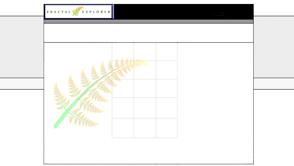
Figure 3.71. Drawing grid.

 

Helpful hint: Use graph paper to draw the fractal by hand. Starting a seed on paper with squares 32 x 16 is most useful. After just a few replacement levels you should start to see a pattern emerge.

 

Figure 3.72 . Ten different patterns produced from sixteen seeds.

 

 

Dragons can also be made using other constructions. Here is one called Spinning Dragon ^[31] that starts out with humble origins that gives the illusion of motion as continuously higher levels are drawn.

 

Figure 3.73 Various levels of the Spinning Dragon.

 

Dragon curves can also be made from IFS as seen in Chapter 6 and L-systems discussed in Chapter 7.

 

 

Growing Fractal Forests and Gardens with Finite Segments and Prepositional Widths (top)

 

" The kingdom of heaven is like a grain of mustard seed, which a man took, and sowed in his field: Which indeed is the least of all seeds: but when it is grown, it is the greatest among herbs, and becometh a tree, so the birds of the air come and lodge in the branches thereof."

Saint Matthew 13: 31,32 from King James Bible

 

As an oak develops from a tiny acorn, so too can a fractal be generated from a simple seed. We will grow fractal: cacti, trees, ferns, plants, along with other items found in nature. Starting from our basic seed shapes we will create increasingly complex objects of nature from successive generations. The true fractal is reached only after an infinite number of generations have been created which in the physical world we can only  approximate. Early generations often give us good approximations of the final fractal picture. Later on we will discuss techniques to speed up fractal generation with greater detail .

Our plants are grown with seeds made with straight lines. This is not as limiting as you might think. With these lines, it is easy to create close approximations to curved fractals as you will see in the next section.

 

The Cactus Plant

The cacti in our garden are an elegant demonstration of how fractals can loose a ridged form and acquire a rounded appearance. All three cactus fractals below are created from straight line seeds with a similar configuration. Their only difference is the progression downward of the two end line's slope.

Figure 3.74 Cactus plants from similar fractal seeds.

 

       Growing a Cactus using  FractaSketch

 

Figure 3.75 The cactus fractal seed in FractaSketch.

Each line segment is replaced by the whole seed in successive generations. The arrowhead denotes orientation. We create the following four generations.

 

Figure 3.76 Cactus going through the following stages of growth.

Now try growing your own fractal cacti and see how changes in line position can effect  your plant's appearance.

 

Growing Trees from Fractal Seeds

" I think that I shall never see, a geometry more beautiful than a tree."  ^[32]

           

            - a slight alteration of Alfred Joyce Kilmer poem Trees (1914)

 

The tree is a prime example of the fractal structure found in plants. To obtain the greatest exposure from air and sunlight, trees of all different sizes and dimensions grow striving to fill space with their branches. Our garden here is in the plane of a computer screen, so we will limit ourselves to trees that approach two-dimensions.

 

 

Trees and Fractals

 

The growth of any plant is not random. It follows given patterns. The branch growth from a tree depends on its species and individual genetic disposition.  As a tree grows its general pattern will stay the same but the length of branches will change depending on the development of the tree crown, the age of the tree, and the varying light conditions which influence the tree's growth.

 

For most trees the growing regions are found in budding areas on a branch. These areas are called the meristem, from the leaves in these areas will develop next year's branches. The location on the branch and the relative distances between the leaves are determined by the tree species. New branches will grow out from these leafed regions resulting in an increased fractal level. The relative length of branches is given by the location of the branch in relation to its next lower order. Without any outside influence, such as physical damage or light competition, the relative growth of these side branches will stay constant.  We will use the branch of a European beech and a branch of an elm tree as templates in the FractaSketch to show how higher order branches can be created. Figure 3.77 shows a European beech branch with 4 levels of replication, its fractal dimension is , and Figure 3.78 shows the elm branch also with 4 levels with fractal dimension of .  More species types can be simulated with this model possibly varying the branch angles.

 

Figure 3.77 Fractal out line of a European beech with  .

 

Figure 3.78 Elm tree branch with .

 

As curtain trees age their crowns become fuller to take greater advantage of their light gathering capabilities for which a more evenly distributed geometry provides. An example is the open crown Acacia often referred to as the " Umbrella Tree" found in Africa. See Figure 3.79 for computer generated Acacia with .

 

Figure 3.79 Acacia or Umbrella Tree with . 

 

In Color Plate 17 and Color Plate 18 you can see some of the different fractal tree structures discussed.

 

Drawing a fractal tree with straight lines is somewhat analogous to building a tree out of 2 x 4 s. In the next section you will get a chance to build trees in such a fashion as well as many others using FractaSketch.

 

Figure 3.80 The blueprints to building a tree.

 

 

       Basic Tree Construction with  FractaSketch

 

Lets draw a tree with the following seed created in FractaSketch see below.

 

Figure 3.81 This "Y" seed is the most basic construction for a fractal tree.

 

Hint: it is easiest to construct a fallen tree, this is a tree laying 90° on its side. Then when the construction is completed you can use the "Rotate" feature from the "Scale" menu to put it in an upright position, see below.

 

Figure 3.82 This is tree's side drawing and its corresponding upright rotation.

 

Lets begin construction of our fallen tree with 3 segments:

           

Step 1: Chose Box 9, the non replaced line segment and draw a horizontal line roughly half way across the screen and click. This will be the tree's trunk.

 

Step 2: Chose Box 1 and draw the tree's first branch. This is done by drawing a line from the trunk with an ascending 45° toward the upper right.

 

Step 3: Chose Box 0, use this to back track invisibly to the top of tree trunk( or in our case the right-hand side). These light gray lines are used to let us draw figures that consist of non continuous or disconnected sections. In this case we use this feature to allow us to draw a symmetric branch on the opposite side.

 

Step 4: Preceded by choosing Box 2. Next draw a line equal in length to the other branch, only this time it should descend by 45° toward the lower left. This "branch" should be symmetric about the tree trunk.

           

Step 5: Choose Box 0, finish the drawing by double clicking and rotate the tree into an upright position. When finished if the "Edit" menu is set to "Left to Right" an invisible line will be automatically drawn to the tree's middle top, this will define the seeds length. Otherwise if the "Edit" menu is set to "First to Last" this will be ignored.

           

 

Lets grow our tree starting at level 1. This image should look like a giant "Y". Proceed to higher levels. See how our stick figure tree is taking shape.

 

In nature, a tree's construction has a supportive structure. Its trunk will generally be longer and proportionally thicker than the connected branches. Trees use this principle to allow the trunk to support the limbs that hold the leaves. A tree needs this large area in order to capture a sufficient amount of sunlight required for photosynthesis.

 

Our trees can also be viewed with line thicknesses proportional to segment lengths. This feature can be use by selecting the "Proportional" command from the "Line" menu ^[33] . This function can be repeated several times to reach a desired width. View the fractal tree you have created at different proportional widths and see which ones look closest to trees you know see below.

 

Figure 3.83 Our basic tree with varying proportional widths.

 

I know, I know you're saying what tree looks like the one we have just drawn. Well there is at least one tree ^[34] that comes close. It is found in the Joshua Tree National Park in California, USA see figure 3.84 on the next page.

 

Figure 3.84  Joshua tree, Joshua Tree National Park, California © 1989 Ken Crounse, Dynamic Software.

 

Another classic fractal tree is the 'bush', created with 8 seed lines. Its dimension is . See Figure 3.81.

 

Figure 3.85 The Bush show here with its seed.

 

Here are some templates and results of familiar trees. You can create your own fractal trees and see what you come up with.

 

Figure 3.86 Recognizable structures of familiar trees.

 

Trees have different fractal structures that adapt to various needs. Next time you are in a place with a large verity of trees, you might take look at  the diversity of trees and categorize them according to their fractal dimension.

 

       The Trees of Hildesheim.

 

 

In the northern region of Germany, trees proudly exhibit their barren fractal structure until late spring. Nestled in this region is the town of Hildesheim, here one can see rows upon rows of leafless trees. These trees, with their striking dark outlines, often accentuated by golden wheat fields, fading hills and a flowing sky look remarkably close to tree structures created by FractaSketch. In fact these trees look so much so, we thought it might be fun to add them to the landscape. Can you find the fractal forgeries in the picture, see Color Plate 19.

 

Figure 3.87 A Euphorbia plant with varied branching structure.

 

Other trees and plants exhibit different structures. In Color Plate 20 and Color Plate 21 you can compare examples of plants with different fractal structures. The first plant exhibits a standard branching with 1 segment dividing into 2 segments that again divides into 2 also seen in Figure 3.86, while the second has a branching structure where 1 segment divides into 2 segments that then divides into 25 segments which again divides into 20 segments as seen in the Euphorbia plant in Figure 3.87. Each structure seems adapted to a special purpose, the first plant desiring to grow outward while the second plant tries to create a large outer budding surface with a minimal amount of structural support.

 

Fractal Ferns in Our Forest

 

Figure 3.88  Bracken Fern, Sierra Nevada, California © 1989 Michael McGuire ^[35]

 

" So much from so little, its beauty lay in simplicity."

 

                                                                                    -Dr. D. von Tischtiegel ^[36]

 

Ferns are one of the most beautiful structure found in nature. On close examination one can see that a fern will not only repeat itself at several levels of magnification but does so with great simplicity. The structure of most ferns can be constructed from four lines of information ^[37] . For these reasons, it has become a common picture found in books on fractals. We will grow one in our book too. Start with the following seed.

Figure 3.89 A basic fern seed.

At first we get growths that look more like ears of wheat than ferns. These self-similar seeds aid in constructing a variety of shapes.

As a fern grows to higher and higher levels, it begins to take its familiar shape as seen below.

Figure 3.90 Growing levels of a fern.

 

In order to speedup computational speed and produce a more evenly distributed fractal, we limit the shortness of each line segment to a curtain number of pixels.

 

The fern ^[38]   below is generated until a 5-pixel line length is reached. Also it is drawn with line thicknesses corresponding to each lines length.

 

Figure 3.91 A fully developed fern with a minimum 5 pixel line length.

 

"The full grown fern is a marvel to behold" - Peter van Roy

 

The fractal fern can also be created by using iterated functions systems or collage methods see Chapter 6.

 

The Maple Leaf's Different Seasons.

 

The maple leaf fractal is an example of an intricate object that has a compelling mixture of order and apparent randomness. It is hard to create fractals with just the right proportions of order and randomness to be pleasing to the eye. In that sense, creating fractals from seeds is like composing a musical score: achieving the best effect requires mastery. Lots of practice and examples of good pictures are needed to gain a true insight. For example, consider the maple leaf seed. Initially it looks more like a high speed plane then a leaf see below.

 

Figure 3.92 The maple leaf seed.

 

 Notice: the dark gray lines are drawn by Boxes 5-8. These line tools invert the picture when drawing. The light gray line of Box 0 lets us draw disconnected figures, discussed in FractaSketch manual section.

 

Through the apparent magic of fractal transformations this is what our full grown object becomes.

 

Figure 3.93 The changing seasons of our maple leaf.

 

 

 The fractals in our forest show the variety of shapes that can result by using the simple recipe of replacing line segments with miniature copies of the whole shape. We have only just begun to explore the richness of the world of fractal geometry. In Chapter 4 we will discuss discus various ways to calculate the fractal dimension of the objects including many of the images we have created here.

 

Coral reefs exhibit fractal branching that is exhibited in aggregate growth fractals. Sea cucumbers do fractal food gathering.  There is a species that has an antenna that branches and fills space like a tree.  When enough food is captured in the tree, it is folded into a rope-like structure (a bunch of strands, one dimensional) and put into the creature's mouth. The change of dimension is very useful for gathering food: as a tree, it can capture lots of plankton, as a rope, it is easily put into the mouth. A Nautilus of the sea uses self-similar growth patterns to expand its habitat in continually larger stages.

 

Figure 3.94 A sea cucumber that uses a transformation of a linear fractal to gather food.

 

Figure 3.95 A Nautilus of the sea and a similar structured linear fractal, just one of a infinite number left for you to explore.

 

For a wide range of other fractals created straight line seeds as in this chapter see fractal gallery  found in Appendix B.